Posts Tagged ‘tetration’

Climbing the ladder of hyper operators: tetration

January 5, 2015 by George Daccache. 17 comments

Arguably the first math lesson we’ve had – ever – dealt with counting. Soon, we’re exposed to addition, and later, multiplication. Finally, when we’re fresh into middle school, we take on exponentiation. And every step of the way, we learn that each new operator is shorthand for repeatedly applying the previous one: addition as repeated counting, multiplication as repeated addition, and exponentiation as repeated multiplication. We quickly see that the above operations can be formalized as follows:

0. Succession: $ a’ = a + 1$

1. Addition: $A(a, b) = a + b = \underbrace{a + 1 + 1 + \cdots + 1}_{b \: times} = \underbrace{(a’)’\cdots’}_{b \: times}$
2. Multiplication: $M(a, b) = a \times b = \underbrace{a + a + a + \cdots + a}_{b \: times}$
3. Exponentiation: $E(a, b) = a^b = \underbrace{a \times a \times a \cdots \times a}_{b \: times}$

Several natural questions spring to mind: Can’t we continue this sequence of operators? Can’t another operator be defined as repeated exponentiation, and can’t we repeat that to get a new operator, ad infinitum? The answer is a resounding yes! In fact, the first such an operator already exists and has several applications in various fields: the tetration operator.

Definition:

Tetration is defined as, $$T(a, b) = {}^ba = \underbrace{a^{a^{a^{…^{a}}}}}_{b \> times}$$ As is readily seen, the notation is the exact same as exponentiation, but with the ‘exponent’ to the left. For the sake of this article, we’ll refer to tetration $n$ times as nth order tetration. That is, if $b$ in the definition is equal to $2$, then it is 2nd order tetration, and so on.

Before we go any further, we must specify how to compute values with the tetration operator, as the notation for repeated exponentiation might lead to a certain measure of ambiguity in that regard. For example, given ${}^4 3$, the definition rewrites it as, $$3^{3^{3^3}}.$$ Is this equal to $$((3^3)^3)^3$$ or $$3^{\left[3^{\left(3^3\right)}\right]}?$$ It happens that the second expansion is the correct one, as tetration is defined as right associative, which means it simplifies from the innermost nesting outward. Thus the value of ${}^4 3$ is, $${}^4 3 = 3^{\left[3^{\left(3^3\right)}\right]} = 3^{\left(3^{27}\right)} = 3^{7625597484987}.$$

To put this number into perspective, the above number has approximately $3.638 \times 10^{12}$ digits, or somewhere over 3 trillion.

Tetration Functions:

In many cases, it is advantageous to define the family of tetration functions so that $t_n(x) = {}^nx$. The most common functions in this family are $t_2(x) = {}^2x = x^x$, and $f_3(x) = {}^3x = x^{x^x}$. Using Wolfram|Alpha, I was able to quickly make two graphs of $t_2(x)$, shown below:

$plot1$

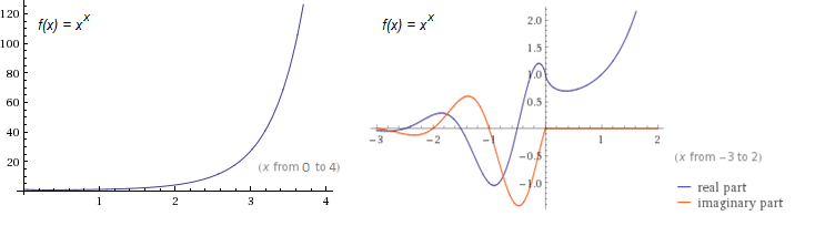
From the first plot, we note just how fast $t_2(x)$ grows. (Its exponential counterpart, $f(x) = 2^x$, is only $16$ at $x = 4$, whereas $t_2(x)$ is already $256$.) From the second, we see the function’s complex behavior for negative $x$. The only points where $t_2(x)$ is real for negative values are precisely at the negative integers.

We also note from the second plot how purely real $t_2(x)$ decreases over a small interval. It is left to the reader as a simple calculus exercise to verify that the real interval where the $t_2(x)$ decreases is $(0, 1/e)$. It happens that this decreasing behavior occurs for all $t_n(x)$, where $n$ is even. A plot of $t_n(x)$ as $n \to \infty$ verifies this.

$plot2$

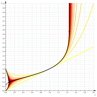
Instantly remarkable from the graph is how half of the functions tend to $1$ as $x$ tends to $0$, and the other half tend to $0$. In fact, we have, $$\lim_{x \to 0^+} t_n(x) = \begin{cases} 1 & \text{if } n \text{ even} \\ 0 & \text{if } n \text{ odd} \end{cases}$$

Growth of Tetration:

From the previous graphs and calculations it is immediately obvious that tetration outputs very large numbers in exchange for very small ones, on an order even larger than its predecessor, exponentiation. It seems reasonable to hope that we can prove that its growth rate dominates that of exponentials. Let’s take a look at the following theorem which does just that.

Theorem: for all $x$ and all $a > 1, b \geq 2$, we have $a^x = o({}^bx)$.

Proof: By definition, we have $a^x = o({}^bx) \Leftrightarrow \lim_{x \to \infty} \frac{a^x}{{}^bx} = 0$. Thus, it suffices to prove the limit for all $a > 1$ and $b \geq 2$: With a quick rewrite in terms of exponentials and logarithms, we have, $$\lim_{x \to \infty} \frac{a^x}{{}^bx} = \lim_{x \to \infty} \exp{\left(x\ln{\left(\frac{a}{{}^{b-1}x}\right)}\right)}$$ $$ = \exp{\left(\lim_{x \to \infty}x \lim_{x \to \infty}\ln{\left(\frac{a}{{}^{b-1}x}\right)}\right)}$$ Clearly the first limit is infinity, but the second limit isn’t as obvious. We argue as follows:

Since it is trivial that tetration increases without bound towards infinity, we have $\lim_{x \to \infty} {}^n x = \infty$. It follows that $\lim_{x \to \infty} \frac{a}{{}^n x} = \frac{a}{\infty} = 0$, becoming increasingly small and staying positive. We know that $\ln{(x)} < 0$ in the range $0 < x < 1$, and so we conclude that $\lim_{x \to \infty} \ln{(a/{}^{b-1}x)} = -\infty$.

We can now directly compute the limit: $$\exp{\left(\lim_{x \to \infty}x \lim_{x \to \infty}\ln{\left(\frac{a}{{}^{b-1}x}\right)}\right)} = e^{[(\infty) \cdot (-\infty)]} = e^{-\infty} = 0.$$ Q.E.D.

Properties of Tetration:

Unfortunately, tetration defies simple rules such as $a^b \cdot a^c = a^{b + c}$, but that doesn’t mean that there aren’t any rules at all. What is hard about deriving properties of tetration is that intuition is not able to play a major role, since no one has a ‘feel’ for tetration as they do for exponentiation. If we restrict ourselves to second-order tetration, however, we find several interesting properties, the most important of which I have stated below.

Property 1 (addition rule of tetration):

$${}^2(a + b) = (a + b)^a \cdot (a + b)^b$$

Property 2 (multiplication rule of tetration):

$${}^2(ab) = {}^2a^b \cdot {}^2b^a$$

Property 3 (hyperbolic rule of tetration):

$${}^2x = \sinh{(x \ln{(x)})} + \cosh{(x \ln{(x)})}$$

While theorems 1 and 2 seem reasonable, theorem 3 seems completely out of the blue. In fact, the theorem both relates tetration to the hyperbolic functions and also provides a way of expressing second order tetration without actually using tetration! Below is the derivation:

Proof:

Start with the relation,

$$e^\theta = \sinh{(\theta)} + cosh{(\theta)}$$

Substitute $\theta = \ln{({}^2x)}$ into the equation and simplify:

$$e^{\ln{({}^2x)}} = \sinh{( \ln{({}^2x)})} + \cosh{(\ln{({}^2x)})}$$

$$ \implies {}^2x = \sinh{(x \ln{(x)})} + \cosh{(x \ln{(x)})}$$

Q.E.D.

To my knowledge, I have never seen any of the above theorems appear in literature on the subject; I derived them myself.

Heading to Arbitrary Bases and Orders:

From the definition of tetration, we see that it can easily be extended to arbitrary bases: ${}^3 0.2$ is easy enough to compute, provided you express it in terms of exponentiation first. The questions, “What is ${}^{-1}2$? Or ${}^{0.25}6$?”, however, are not as easy to answer. This question about extending nth order tetration to arbitrary heights, or orders, is the elephant in the room of unsolved questions about this hyper operator. (An analogue of this question would be how to extend factorials to the reals, with the gamma function being the answer.)

Till now, there is no general consensus on tetration’s extension to arbitrary or even negative heights, but there are several competing theories, all with varying levels of difficulty. Perhaps the easiest approach to understand is that of Daniel Geisler, founder of the webpage tetration.org, who attempts to rectify the problem using Taylor series. Another very promising approach given by Kneser much earlier was proven to be both real analytic and unique and works by constructing an Abel function of $e^x$ and using a Riemann mapping. As the scope of this article is meant to be for undergraduates and/or very bright high school attendees, I shall not discuss the detailed procedures in the constructions but will give links to relevant sources at the end.

Applications:

For many, it is enough to study the properties of tetration simply because of its existence, but for the more applied of the readers among you, it might come as a relief to find out that both tetration and its inverse (and variants thereof) find application in many areas, with other fields also being candidates for its use.

Starting from mathematics itself, one finds that the modern version of the Ackermann function is actually equal to base-two nth order tetration, and can thus help in easily expressing the outputs of such a function. We have,

$${}^n2 = A(4, n-3) + 3.$$

(Note: This $A(a, b)$ is the Ackermann function, and not the “addition” function given at the beginning of the article, even though they both are denoted $A$.)

The original three-argument version of Ackermann’s function gives rise to tetration more generally:

$$φ(a, b, 3) = {}^ba.$$

Note that the Ackermann function is discrete, so finding a continuous version of the function is equivalent to extending tetration to all heights.

Another application is in computing the number of elements in the Von Neumann universe construction in set theory: the number is ${}^2n$, where here $n$ is the stage of the construction. It serves as an aid in understanding the rapid growth of the elements in each stage.

If one considers the inverse function of second order tetration, called the super square root $\text{ssrt(}x\text{)}$, we find several other applications, mentioned below.

Define $$\text{wzl(}x\text{)} = \text{ssrt(}10^x\text{)}$$ This function is called the ‘wexzal’ (a modification of the German word for ‘root’), and was coined and studied extensively in the self-titled paper, found below. According to the paper, using plotting software and extensive numerical tables for comparison, the authors found a more accurate equation for modeling velocity decay in ballistics which is the equation, $$v = \frac{a}{\text{wzl(}e^{bx}\text{)}}$$ as apposed to the traditional equation, $$v = \frac{a}{e^{bx}}.$$ Note that $a$ and $b$ are parameters depending on each case. This new equation also has the advantage of being integrable to find the flight time, so nothing is lost from the less accurate equation’s advantages.

Similarly, we can find using this variation of tetration’s inverse significantly better fits for various firearm quantities such as muzzle velocity as well as for motor vehicle acceleration.

Conclusion

So what’s the whole point of this? This article serves as a reminder that there are many areas of mathematics left untouched despite the vast compendium we have now. It simply examines one such unturned rock and gives a look into possible developments into the theory of hyper operators. Regrettably, some topics were not discussed for the sake of brevity, such as tetration’s inverse operation and calculus with the tetration function. For the eager reader, though, I have included some resources to further knowledge on the subject.

current community

more communities