Green’s Theorem and Area of Polygons

A common method used to find the area of a polygon is to break the polygon into smaller shapes of known area. For example, one can separate the polygon below into two triangles and a rectangle:

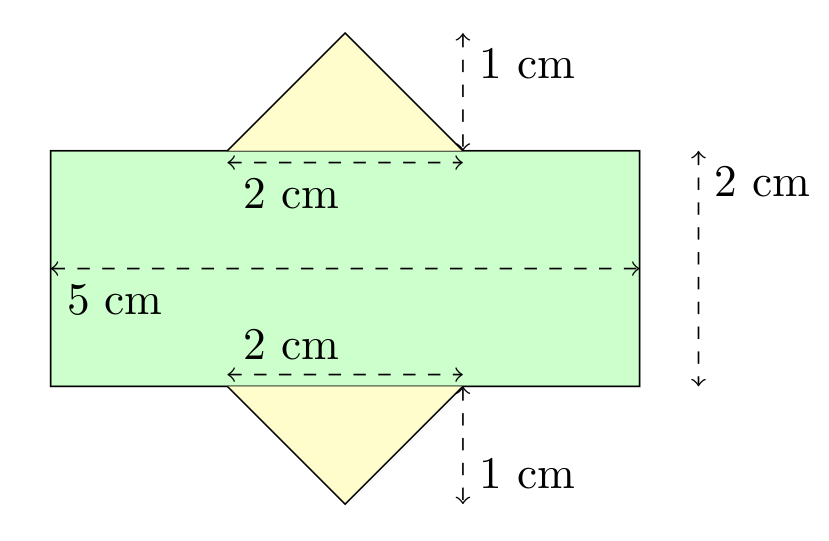
By breaking this composite shape into smaller ones, the area is at hand: $$\begin{align}A_1 &= bh = 5\cdot 2 = 10 \\ A_2 = A_3 &= \frac{bh}{2} = \frac{2\cdot 1}{2} = 1 \\ A_{total} &= A_1+A_2+A_3 = 12\end{align}$$

Unfortunately, this approach can be difficult for a person to use when they cannot physically (or mentally) see the polygon, such as when a polygon is given as a list of many vertices.

Formula

Happily, there is a formula for the area of any simple polygon that only requires knowledge of the coordinates of each vertex. It is as follows: $$A = \sum_{k=0}^{n} \frac{(x_{k+1} + x_k)(y_{k+1}-y_{k})}{2} \tag{1}$$ (Where \({n}\) is the number of vertices, \({(x_k, y_k)}\) is the \({k}\)-th point when labelled in a counter-clockwise manner, and \({(x_{n+1}, y_{n+1}) = (x_0, y_0)}\); that is, the starting vertex is found both at the start and end of the list of vertices.)

It should be noted that the formula is not “symmetric” with respect to the signs of the \({x}\) and \({y}\) coordinates. This can be explained by considering the “negative areas” incurred when adding the signed areas of the triangles with vertices \({(0,0)-(x_k, y_k)-(x_{k+1}, y_{k+1})}\).

In the next sections, I derive this formula using Green’s Theorem, show an example of its use, and provide some applications.

Derivation

Green’s Theorem states that, for a “well-behaved” curve \({C}\) forming the boundary of a region \({D}\):

\(\displaystyle \oint_C P(x, y)\;\mathrm dx + Q(x, y)\;\mathrm dy = \iint_D \frac{\partial Q}{\partial x} – \frac{\partial P}{\partial y}\;\mathrm dA \ \ \ \ \ (2)\)

(In this context, “well behaved” means, among other things, that \({C}\) is piecewise smooth. For a full listing of the requirements for \({C}\) and \({D}\), please see here.)

Recalling that the area of \({D}\) is equal to \({\iint_D \;\mathrm dA}\), we can use Green’s Theorem to calculate area if we choose \({P}\) and \({Q}\) such that \({\frac{\partial Q}{\partial x} – \frac{\partial P}{\partial y}=1}\). Clearly, choosing \({P(x, y) = 0}\) and \({Q(x, y) = x}\) satisfies this requirement.

Thus, letting \({A}\) be the area of the region \({D}\):

\(\displaystyle A = \oint_C x\;\mathrm dy \ \ \ \ \ (3)\)

Now, consider the polygon below, bordered by the piecewise-smooth curve \({C = C_0\cup C_1\cup\cdots\cup C_{n-1}\cup C_n}\), where \({C_k}\) starts at the point \({(x_k, y_k)}\) and ends at the “next” point along the polygon’s edge when proceeding counter-clockwise. (N.B. If we proceed in a clockwise manner, we get the negative of the area of the polygon.)

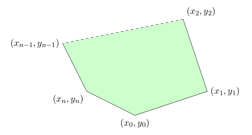
Note: the dashed lines indicate that there could be any number of points between \({(x_2, y_2)}\) and \({(x_{n-1}, y_{n-1})}\); this is a complete polygon.

Because line integrals over piecewise-smooth curves are additive over length, we have that:

\(\displaystyle A = \oint_C x\;\mathrm dy = \int_{C_0} x\;\mathrm dy + \cdots + \int_{C_n} x\;\mathrm dy \ \ \ \ \ (4)\)

To compute the \({k}\)-th line line integral above, parametrize the segment from \({(x_k, y_k)}\) to \({(x_{k+1}, y_{k+1})}\):

\(\displaystyle C_k:\; \vec{r}=\left((x_{k+1} – x_k)t + x_k,\; (y_{k+1} – y_k)t + y_k\right),\quad 0\le t\le 1 \ \ \ \ \ (5)\)

Substituting this parametrization into the integral, we find: $$\begin{align}\int_{C_k} x\;\mathrm dy &= \int_0^1 \left((x_{k+1} – x_k)t + x_k\right)\left(y_{k+1} – y_k\right)\;\mathrm dt \\ &= \frac{(x_{k+1} + x_k)(y_{k+1}-y_{k})}{2}\end{align}$$

Summing all of the \(C_k\)’s, we then find the total area: $$A = \sum_{k=0}^{n} \frac{(x_{k+1} + x_k)(y_{k+1}-y_{k})}{2} \tag{6}$$

Example

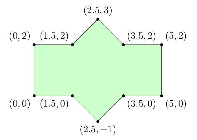
To demonstrate use of this formula, let us apply this to the shape at the beginning of the document. A copy of the image is found below, but this one is marked with the coordinates of the vertices.

Starting with the coordinate \({(0, 0)}\) and proceeding counter-clockwise (again, if we go in the opposite direction, we get the negative of the correct area), we apply our formula:

$$\begin{align} A &= \sum_{k=0}^{n} \frac{(x_{k+1} + x_k)(y_{k+1}-y_{k})}{2} \\ &= \frac{(1.5 + 0)(0 – 0)}{2} + \frac{(2.5 + 1.5)(-1 – 0)}{2} + \frac{(3.5 + 2.5)(0 – (-1))}{2} + \frac{(5+3.5)(0-0)}{2} \\ &\quad + \frac{(5+5)(2-0)}{2} + \frac{(3.5+5)(2-2)}{2} + \frac{(2.5+3.5)(3-2)}{2}\\ &\quad +\frac{(1.5+2.5)(2-3)}{2} + \frac{(0+1.5)(2-2)}{2} + \frac{(0+0)(0-2)}{2}\\ &= 0 + (-2) + 3 + 0 + 10 + 0 + 3 + (-2) + 0 + 0\\ &= 12 \end{align}$$

We arrive at the same answer we had above, which is good. (Obviously!)

Possible Applications

Although this formula is an interesting application of Green’s Theorem in its own right, it is important to consider why it is useful. As can be seen above, this approach involves a lot of tedious arithmetic. Thus, its main benefit arises when applied in a computer program, when the tedium is no longer an issue.

From an engineering perspective, this formula could be used to determine the area (and, using similarly-derived formulas for the moments of a polygon about the \({x}\) and \({y}\) axes, the centroid) of component in a CAD program. Many computer programs estimate all shapes as polygons or connected line segments (rather than exact curves/circles), which means this formula can be directly applied to the existing representation in software.

In a contrived context, this formula can also be useful in collegiate programming competitions. (This was why I first took note of this formula.) Some problems in the “computational geometry” category may involve computing the area of specific polygons, such as the convex hull of a set of points. Knowing the derivation can make it easier to recall during a competition event.

As a final example, one can use this formula to approximate the area of a plot of land. Over a small region, surface area on a sphere can be approximated as that on a rectangle. Thus, an irregularly-shaped plot of land can be modelled as an polygon. Once coordinates are established for each vertex, the formula derived above can be applied to find its area.