Introduction

Every so often, the question comes up (either here or elsewhere) of why induction is a valid proof technique. And this is of course a very natural question. Induction is after all rather mysterious compared to the other usual proof techniques. At the same time, it is a very useful one, so it is important that people can be given a satisfactory answer. The question is more precisely “why can we do induction on the natural numbers”, but I am not going to answer that question here. For one thing, the answer depends entirely on how one defines the natural numbers, and for another, induction has nothing to do with the natural numbers. “But wait” you might say. “Did he really just claim that induction has nothing to do with the natural numbers. How can that be? Is induction not something like, we prove something holds for \({0}\) and that if it holds for \({n}\) then it holds for \({n+1}\). How does that even make sense if we are not talking about the natural numbers?” And indeed, the “nothing” was a bit of an overstatement to get your attention. But it turns out that induction is a proof technique that can be used in a much more general setting than that of the natural numbers. This is the viewpoint I will try to explain in detail in this post: Given some set \({X}\), what do we need to be able to use induction to prove that something holds for all elements of \({X}\)?

The usual case

To get started, let us look at the way induction is usually formulated (I will formulate this as a theorem, but as mentioned, I will not give a proof).

Theorem Let \({A\subseteq {\mathbb N}}\) such that \({0\in A}\) and for all \({n\in {\mathbb N}}\) we have \({n\in A\implies n+1\in A}\). Then \({A = {\mathbb N}}\).

At first glance, it seems like this uses some special properties of the natural numbers, namely the facts that we have a \({0}\) and a way to add \({1}\) to any element. But let us look at a different version of induction (often called “strong” induction). Often, we are told that this version is “equivalent” to the usual induction. But as will be seen later, this is either trivial (as both are true statements about the natural numbers), or false (as the theorems do not hold for the same sets when we start to generalize).

Theorem Let \({A\subseteq {\mathbb N}}\) such that for all \({n\in {\mathbb N}}\) we have \({\left(m < n \implies m\in A\right)\implies n\in A}\). Then \({A = {\mathbb N}}\).

(Note that I have the “baseless” version here. But clearly any set satisfying the above will contain \({0}\) since if \({n=0}\) then \({m < n}\) is always false and hence the first implication becomes true regardless of whether \({m\in A}\), which means that the second implication can only be true if \({n\in A}\)). So now we have a version of induction that only uses the ordering of the natural numbers, and this seems like it might be easier to generalize. So let us take a set \({X}\). What sort of ordering must we put on \({X}\) in order to be able to prove that something holds for all \({x\in X}\) by induction? The common answer is “a well-order”, but this is not quite correct, mainly because a well-order is a total order, and it turns out that it is possible to use induction with just a partial order. But let us still start with the more specific question: What sort of total order on \({X}\) allows us to do induction?

Total orders

In this case, the answer is indeed “a well-order”. So let us first look at the definition.

Definition A total order on a non-empty set \({X}\) is called a well-order if any non-empty subset of \({X}\) has a smallest element.

So my claim is that if \({X}\) is a totally ordered set, then we can do induction on \({X}\) if and only if \({X}\) is well-ordered. But this then refers to the “strong” induction. What happened to the other kind? Can we make sense of the other kind if we just have a total order? The answer to the last question is: Almost. If we have a well-ordered set (with a small additional condition), then we can in fact make sense of the usual kind of induction. But it need no longer be a true statement, unless we change some details. Before we move on to the first kind of induction, let us prove the above claim that being well-ordered is both necessary and sufficient. First, we prove that if is sufficient.

Theorem Let \({X}\) be a well-ordered set and \({A\subseteq X}\) be such that for all \({x\in X}\) we have \({\left(y < x \implies y\in A\right)\implies x\in A}\). Then \({A = X}\).

Proof: Let \({B = X\setminus A}\) and assume for the purpose of contradiction that \({B}\) is not empty. Since \({X}\) is well-ordered this means that \({B}\) has a smallest element, call it \({b}\). But now, if \({x\in X}\) with \({x < b}\) then \({x\not\in B}\) since \({b}\) was smallest in \({B}\). Hence for all \({x\in X}\) with \({x < b}\) we have \({x\in A}\), and thus by the assumption on \({A}\), this means that \({b\in A}\) contradicting the choice of \({b}\). \(\Box\)

And then that it is necessary.

Theorem Let \({X}\) be a totally ordered non-empty set such that whenever a subset \({A\subseteq X}\) satisfies \({\left(y < x \implies y\in A\right)\implies x\in A}\) for all \({x\in X}\) then \({A = X}\). Then \({X}\) is well-ordered.

Proof: Let \({B\subseteq X}\) be a subset and assume that \({B}\) does not have a smallest element. Let \({A = X\setminus B}\). We need to show that \({A = X}\) and thus by assumption it is enough to show that if \({x\in X}\) and \({y\in A}\) for all \({y < x}\) then \({x\in A}\). But if \({y\in A}\) for all \({y < x}\) then \({x}\) cannot be in \({B}\), since it would then be the smallest element in \({B}\) (since all strictly smaller elements are not in \({B}\)), and thus \({x\in A}\) as we needed. \(\Box\)

So now the question remains how we can make sense of the first kind of induction, where we needed to have a \({0}\) and needed to be able to add \({1}\) to any element. But there is a very natural way to make sense of these things in a well-ordered set \({X}\), if we just assume one extra thing: \({X}\) does not have a largest element. Namely, we can take \({0}\) to be the smallest element of the set (which exists by assumption). As for adding \({1}\), this really just means “take the next element”, and this makes sense since for any \({x\in X}\) we know that the set \({\{y\in X\mid y > x\}}\) is non-empty (this is where we need \({X}\) to not have a largest element), and thus it has a smallest element, which is the “next” element after \({x}\) (called the immediate successor of \({x}\)). So with these definitions in hand, given a well-ordered set \({X}\) which does not have a largest element, can we do induction on \({X}\)? The answer turns out to be “no”, as the following example demonstrates. The example also illustrates what we need to change to make things work.

Example Let \({X = \{0,1\}\times {\mathbb N}}\) and order \({X}\) lexicographically (so \({(m,n) \leq (m’,n’)}\) if \({m < m’}\) or \({m = m’}\) and \({n\leq n’}\)). It is then easy to check that \({(0,0)}\) is the smallest element of \({X}\) (i.e. we denote \({0 = (0,0)}\)). It is also easy to check that with “\({+1}\)” defined as explained above, we have \({(m,n)+1 = (m,n+1)}\). Let \({A = \{(0,n)\mid n\in {\mathbb N}\}\subseteq X}\). Then the above observations show that \({0\in A}\) and \({a\in A\implies a+1\in A}\) but \({A\neq X}\). But \({X}\) is indeed well-ordered (this is a standard exercise that I leave to the reader), so this is a well-ordered set without a largest element where we cannot use the first kind of induction.

So what is it that goes wrong in the above example? If we look at the usual proof of why induction works for the natural numbers, it is very close to the proof I have presented here that “strong” induction works on any well-ordered set, except that at one point, one will need that if \({n\neq 0}\) then \({n-1}\) makes sense (one considers the complement of the given set, takes the smallest element \({n}\) and notices that this cannot be \({0}\) and then uses the inductive assumption on \({n-1}\)). But how would we define “subtract \({1}\)” in a general well-ordered set? This turns out to not be doable, and this is precisely what goes wrong in the example. More precisely, “subtract \({1}\)” should mean “take the immediate predecessor”, and such need not exist. In the given example, the element \({(1,0)}\) does not have any immediate predecessor, since the elements smaller than \({(1,0)}\) are precisely those in the chosen set \({A}\), and an immediate predecessor would be a largest element in \({S}\), which clearly does not exist. The above suggests how we can remedy the situation: Replace “\({0\in A}\)” by “\({x\in A}\) for any \({x\in X}\) which does not have an immediate predecessor”. And indeed, with this version, we can do induction (I leave the proof as an exercise to the reader. It is just a small change compared to the other proof given).

Partial orders

Back to the more general case: Let \({X}\) be a partially ordered set. What do we need to assume about this partial order in order to do induction on \({X}\) (from now on, by induction I will mean “strong” induction since we cannot really make sense of the other kind in this larger generality). Here the answer turns out to be that we need \({X}\) to be well-founded (actually we do not need an ordering, just any well-founded relation, but I will stick with an ordering). So let us define this.

Definition A partially ordered non-empty set \({X}\) is said to be well-founded if any non-empty subset of \({X}\) has a minimal element.

Let us as previously prove that this condition is both sufficient and necessary to do induction. First, sufficient.

Theorem Let \({X}\) be a well-founded partially ordered set and \({A\subseteq X}\) such that for all \({x\in X}\) we have \({\left(y < x \implies y\in A\right)\implies x\in A}\). Then \({A = X}\).

Proof: Let \({B = X\setminus A}\). Assume for the purpose of contradiction that \({B}\) is not empty, and let \({b\in B}\) be a minimal element. Now it is clear that if \({x\in X}\) with \({x < b}\) then \({x\in A}\) since otherwise \({b}\) would not be minimal. But then \({b\in A}\) contradicting the choice of \({b}\). \(\Box\)

And necessary.

Theorem Let \({X}\) be a partially ordered non-empty set such that whenever a subset \({A\subseteq X}\) satisfies \({\left(y < x \implies y\in A\right)\implies x\in A}\) for all \({x\in X}\) then \({A = X}\). Then \({X}\) is well-founded.

Proof: Let \({B\subseteq X}\) and assume that \({B}\) does not have a minimal element. Let \({A = X\setminus B}\). Now if \({x\in X}\) and \({y\in A}\) for all \({y < x}\) then also \({x\in A}\) as otherwise \({x}\) would be a minimal element of \({B}\). But then by assumption, \({A = X}\) so \({B}\) is empty. \(\Box\)

So now we know when we can do induction. But is this ever useful? And it sure is! For a concrete example of a well-founded set with a non-total order, we can take \({{\mathbb Z}}\) with the ordering \({m\leq n}\) if \({m = n}\) or \({|m| < |n|}\) (the “closer to zero” ordering). Sure, we could also mess a bit with the ordering to make it total, but this makes for a simpler description (for an example where this ordering is used, see my answer here). A useful and easy result for proving that certain sets are well-founded is the following.

Proposition Let \({X}\) be a partially ordered non-empty set such that for all \({x\in X}\), the set \({ \{y\in X\mid y\leq x \} }\) is finite. Then \({X}\) is well-founded.

Proof: Let \({A\subseteq X}\) be a non-empty subset and let \({a\in A}\). Now the set \({ \{x\in X\mid x\leq a \} \cap A}\) is finite and non-empty and thus has a minimal element, which is a minimal element in \({A}\). \(\Box\)

An exercise for the readers

Finally, to end the post, I have an exercise for the readers. Go and find good examples of proofs by induction where the set in question is not the natural numbers. Even better, find ones where the set in question is not the natural numbers, but where the proof ended up being more complicated because the author has taken pains to only do induction on the natural numbers (this need not reflect poorly on the author. If the proof is meant for inexperienced people, then it is often better to give the less direct proof which uses the sort of induction the readers will be familiar with). Go ahead and fill the comments with such examples.

While teaching a largely student-discovery style elementary number theory course to high schoolers at the Summer@Brown program, we were looking for instructive but interesting problems to challenge our students. By we, I mean Alex Walker, my academic little brother, and me, David Lowry-Duda. After a bit of experimentation with generators and orders, we stumbled across a proof of Wilson’s Theorem, different than the standard proof.

Wilson’s theorem is a classic result of elementary number theory, and is used in some elementary texts to prove Fermat’s Little Theorem, or to introduce primality testing algorithms that give no hint of the factorization.

Theorem 1 (Wilson’s Theorem) For a prime number \({p}\), we have $$ (p-1)! \equiv -1 \pmod p. \tag{1}$$

The theorem is clear for \({p = 2}\), so we only consider proofs for “odd primes \({p}\).”

The standard proof of Wilson’s Theorem included in almost every elementary number theory text starts with the factorial \({(p-1)!}\), the product of all the units mod \({p}\). Then as the only elements which are their own inverses are \({\pm 1}\) (as \({x^2 \equiv 1 \pmod p \iff p \mid (x^2 – 1) \iff p\mid x+1}\) or \({p \mid x-1}\)), every element in the factorial multiples with its inverse to give \({1}\), except for \({-1}\). Thus \({(p-1)! \equiv -1 \pmod p.} \diamondsuit\)

Now we present a different proof.

Take a primitive root \({g}\) of the unit group \({(\mathbb{Z}/p\mathbb{Z})^\times}\), so that each number \({1, \ldots, p-1}\) appears exactly once in \({g, g^2, \ldots, g^{p-1}}\). Recalling that \({1 + 2 + \ldots + n = \frac{n(n+1)}{2}}\) (a great example of classical pattern recognition in an elementary number theory class), we see that multiplying these together gives \({(p-1)!}\) on the one hand, and \({g^{(p-1)p/2}}\) on the other.

As \({g^{(p-1)/2}}\) is a solution to \({x^2 \equiv 1 \pmod p}\), and it is not \({1}\) since \({g}\) is a generator and thus has order \({p-1}\). So \({g^{(p-1)/2} \equiv -1 \pmod p}\), and raising \({-1}\) to an odd power yields \({-1}\), completing the proof \(\diamondsuit\).

After posting this, we have since seen that this proof is suggested in a problem in Ireland and Rosen’s extremely good number theory book. But it was pleasant to see it come up naturally, and it’s nice to suggest to our students that you can stumble across proofs.

It may be interesting to question why \({x^2 \equiv 1 \pmod p \iff x \equiv \pm 1 \pmod p}\) appears in a fundamental way in both proofs.

This post appears on the author’s personal website davidlowryduda.com and on the Math.Stackexchange Community Blog math.blogoverflow.com.

Arguably the first math lesson we’ve had – ever – dealt with counting. Soon, we’re exposed to addition, and later, multiplication. Finally, when we’re fresh into middle school, we take on exponentiation. And every step of the way, we learn that each new operator is shorthand for repeatedly applying the previous one: addition as repeated counting, multiplication as repeated addition, and exponentiation as repeated multiplication. We quickly see that the above operations can be formalized as follows:

• 0. Succession: \( a’ = a + 1\)

• 1. Addition: \(A(a, b) = a + b = \underbrace{a + 1 + 1 + \cdots + 1}_{b \: times} = \underbrace{(a’)’\cdots’}_{b \: times}\)
• 2. Multiplication: \(M(a, b) = a \times b = \underbrace{a + a + a + \cdots + a}_{b \: times}\)
• 3. Exponentiation: \(E(a, b) = a^b = \underbrace{a \times a \times a \cdots \times a}_{b \: times}\)

Several natural questions spring to mind: Can’t we continue this sequence of operators? Can’t another operator be defined as repeated exponentiation, and can’t we repeat that to get a new operator, ad infinitum? The answer is a resounding yes! In fact, the first such an operator already exists and has several applications in various fields: the tetration operator.

Definition:

Tetration is defined as, $$T(a, b) = {}^ba = \underbrace{a^{a^{a^{…^{a}}}}}_{b \> times}$$ As is readily seen, the notation is the exact same as exponentiation, but with the ‘exponent’ to the left. For the sake of this article, we’ll refer to tetration \(n\) times as nth order tetration. That is, if \(b\) in the definition is equal to \(2\), then it is 2nd order tetration, and so on.

Before we go any further, we must specify how to compute values with the tetration operator, as the notation for repeated exponentiation might lead to a certain measure of ambiguity in that regard. For example, given \({}^4 3\), the definition rewrites it as, $$3^{3^{3^3}}.$$ Is this equal to $$((3^3)^3)^3$$ or $$3^{\left[3^{\left(3^3\right)}\right]}?$$ It happens that the second expansion is the correct one, as tetration is defined as right associative, which means it simplifies from the innermost nesting outward. Thus the value of \({}^4 3\) is, $${}^4 3 = 3^{\left[3^{\left(3^3\right)}\right]} = 3^{\left(3^{27}\right)} = 3^{7625597484987}.$$

To put this number into perspective, the above number has approximately \(3.638 \times 10^{12}\) digits, or somewhere over 3 trillion.

Tetration Functions:

In many cases, it is advantageous to define the family of tetration functions so that \(t_n(x) = {}^nx\). The most common functions in this family are \(t_2(x) = {}^2x = x^x\), and \(f_3(x) = {}^3x = x^{x^x}\). Using Wolfram|Alpha, I was able to quickly make two graphs of \(t_2(x)\), shown below:

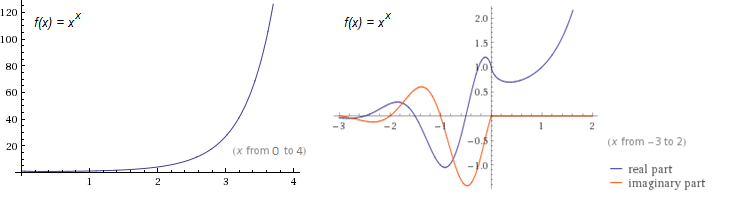
From the first plot, we note just how fast \(t_2(x)\) grows. (Its exponential counterpart, \(f(x) = 2^x\), is only \(16\) at \(x = 4\), whereas \(t_2(x)\) is already \(256\).) From the second, we see the function’s complex behavior for negative \(x\). The only points where \(t_2(x)\) is real for negative values are precisely at the negative integers.

We also note from the second plot how purely real \(t_2(x)\) decreases over a small interval. It is left to the reader as a simple calculus exercise to verify that the real interval where the \(t_2(x)\) decreases is \((0, 1/e)\). It happens that this decreasing behavior occurs for all \(t_n(x)\), where \(n\) is even. A plot of \(t_n(x)\) as \(n \to \infty\) verifies this.

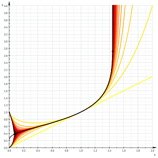
Instantly remarkable from the graph is how half of the functions tend to \(1\) as \(x\) tends to \(0\), and the other half tend to \(0\). In fact, we have, $$\lim_{x \to 0^+} t_n(x) = \begin{cases} 1 & \text{if } n \text{ even} \\ 0 & \text{if } n \text{ odd} \end{cases}$$

Growth of Tetration:

From the previous graphs and calculations it is immediately obvious that tetration outputs very large numbers in exchange for very small ones, on an order even larger than its predecessor, exponentiation.  It seems reasonable to hope that we can prove that its growth rate dominates that of exponentials. Let’s take a look at the following theorem which does just that.

Theorem: for all \(x\) and all \(a > 1, b \geq 2\), we have \(a^x = o({}^bx)\).

Proof: By definition, we have \(a^x = o({}^bx) \Leftrightarrow \lim_{x \to \infty} \frac{a^x}{{}^bx} = 0\). Thus, it suffices to prove the limit for all \(a > 1\) and \(b \geq 2\): With a quick rewrite in terms of exponentials and logarithms, we have, $$\lim_{x \to \infty} \frac{a^x}{{}^bx} = \lim_{x \to \infty} \exp{\left(x\ln{\left(\frac{a}{{}^{b-1}x}\right)}\right)}$$ $$ = \exp{\left(\lim_{x \to \infty}x \lim_{x \to \infty}\ln{\left(\frac{a}{{}^{b-1}x}\right)}\right)}$$ Clearly the first limit is infinity, but the second limit isn’t as obvious. We argue as follows:

Since it is trivial that tetration increases without bound towards infinity, we have \(\lim_{x \to \infty} {}^n x = \infty\). It follows that \(\lim_{x \to \infty} \frac{a}{{}^n x} = \frac{a}{\infty} = 0\), becoming increasingly small and staying positive. We know that \(\ln{(x)} < 0\) in the range \(0 < x < 1\), and so we conclude that \(\lim_{x \to \infty} \ln{(a/{}^{b-1}x)} = -\infty\).

We can now directly compute the limit: $$\exp{\left(\lim_{x \to \infty}x \lim_{x \to \infty}\ln{\left(\frac{a}{{}^{b-1}x}\right)}\right)} = e^{[(\infty) \cdot (-\infty)]} = e^{-\infty} = 0.$$ Q.E.D.

Properties of Tetration:

Unfortunately, tetration defies simple rules such as \(a^b \cdot a^c = a^{b + c}\), but that doesn’t mean that there aren’t any rules at all. What is hard about deriving properties of tetration is that intuition is not able to play a major role, since no one has a ‘feel’ for tetration as they do for exponentiation. If we restrict ourselves to second-order tetration, however, we find several interesting properties, the most important of which I have stated below.

Property 1 (addition rule of tetration):

$${}^2(a + b) = (a + b)^a \cdot (a + b)^b$$

Property 2 (multiplication rule of tetration):

$${}^2(ab) = {}^2a^b \cdot {}^2b^a$$

Property 3 (hyperbolic rule of tetration):

$${}^2x = \sinh{(x \ln{(x)})} + \cosh{(x \ln{(x)})}$$

While theorems 1 and 2 seem reasonable, theorem 3 seems completely out of the blue. In fact, the theorem both relates tetration to the hyperbolic functions and also provides a way of expressing second order tetration without actually using tetration! Below is the derivation:

Proof:

Start with the relation,

$$e^\theta = \sinh{(\theta)} + cosh{(\theta)}$$

Substitute \(\theta = \ln{({}^2x)}\) into the equation and simplify:

$$e^{\ln{({}^2x)}} = \sinh{( \ln{({}^2x)})} + \cosh{(\ln{({}^2x)})}$$

$$ \implies {}^2x = \sinh{(x \ln{(x)})} + \cosh{(x \ln{(x)})}$$

Q.E.D.

To my knowledge, I have never seen any of the above theorems appear in literature on the subject; I derived them myself.

Heading to Arbitrary Bases and Orders:

From the definition of tetration, we see that it can easily be extended to arbitrary bases: \({}^3 0.2\) is easy enough to compute, provided you express it in terms of exponentiation first. The questions, “What is \({}^{-1}2\)? Or \({}^{0.25}6\)?”, however, are not as easy to answer. This question about extending nth order tetration to arbitrary heights, or orders, is the elephant in the room of unsolved questions about this hyper operator. (An analogue of this question would be how to extend factorials to the reals, with the gamma function being the answer.)

Till now, there is no general consensus on tetration’s extension to arbitrary or even negative heights, but there are several competing theories, all with varying levels of difficulty. Perhaps the easiest approach to understand is that of Daniel Geisler, founder of the webpage tetration.org, who attempts to rectify the problem using Taylor series. Another very promising approach given by Kneser much earlier was proven to be both real analytic and unique and works by constructing an Abel function of \(e^x\) and using a Riemann mapping. As the scope of this article is meant to be for undergraduates and/or very bright high school attendees, I shall not discuss the detailed procedures in the constructions but will give links to relevant sources at the end.

Applications:

For many, it is enough to study the properties of tetration simply because of its existence, but for the more applied of the readers among you, it might come as a relief to find out that both tetration and its inverse (and variants thereof) find application in many areas, with other fields also being candidates for its use.

Starting from mathematics itself, one finds that the modern version of the Ackermann function is actually equal to base-two nth order tetration, and can thus help in easily expressing the outputs of such a function. We have,

$${}^n2 = A(4, n-3) + 3.$$

(Note: This \(A(a, b)\) is the Ackermann function, and not the “addition” function given at the beginning of the article, even though they both are denoted \(A\).)

The original three-argument version of Ackermann’s function gives rise to tetration more generally:

$$φ(a, b, 3) = {}^ba.$$

Note that the Ackermann function is discrete, so finding a continuous version of the function is equivalent to extending tetration to all heights.

Another application is in computing the number of elements in the Von Neumann universe construction in set theory: the number is \({}^2n\), where here \(n\) is the stage of the construction. It serves as an aid in understanding the rapid growth of the elements in each stage.

If one considers the inverse function of second order tetration, called the super square root \(\text{ssrt(}x\text{)}\), we find several other applications, mentioned below.

Define $$\text{wzl(}x\text{)} = \text{ssrt(}10^x\text{)}$$ This function is called the ‘wexzal’ (a modification of the German word for ‘root’), and was coined and studied extensively in the self-titled paper, found below. According to the paper, using plotting software and extensive numerical tables for comparison, the authors found a more accurate equation for modeling velocity decay in ballistics which is the equation, $$v = \frac{a}{\text{wzl(}e^{bx}\text{)}}$$ as apposed to the traditional equation, $$v = \frac{a}{e^{bx}}.$$ Note that \(a\) and \(b\) are parameters depending on each case. This new equation also has the advantage of being integrable to find the flight time, so nothing is lost from the less accurate equation’s advantages.

Similarly, we can find using this variation of tetration’s inverse significantly better fits for various firearm quantities such as muzzle velocity as well as for motor vehicle acceleration.

Conclusion

So what’s the whole point of this? This article serves as a reminder that there are many areas of mathematics left untouched despite the vast compendium we have now. It simply examines one such unturned rock and gives a look into possible developments into the theory of hyper operators. Regrettably, some topics were not discussed for the sake of brevity, such as tetration’s inverse operation and calculus with the tetration function. For the eager reader, though, I have included some resources to further knowledge on the subject.

Further Reading and References

• Wexzal paper, discussing quite thoroughly the tetration function and its inverse as well as the wexzal function and its applications.
• Daniel Geisler’s site on tetration and his proposed extension.
• The tetration forum, which hosts mostly higher-level math discussions on tetration and related concepts.
• Kneser’s analytic extension procedure of tetration and its inverse and a proof of its uniqueness
• My own brief research on the properties of second-order tetration.

There are some questions that are really easily posed, have an obvious answer, but are in fact really, really hard to answer in a mathematically satisfactory way. Two examples are:

1. How many holes does a doughnut have?
2. Are a ball and a disk “the same thing”? Meaning: can I deform the first to make it the second in a way that locally preserves its structure, i.e. without tearing, and without “squishing” things too much?

The intuitive (and actually correct) answers are: one, and no. However, in order to prove them true, we’ll have first to formalize the questions in mathematical language, and then to develop a theory that will allow us to work on them.

Let’s start with the first question. “A doughnut” can be interpreted in two ways: it could be a filled doughnut, that is the space \(S^1\times D^2\), where \(S^1\) denotes the circle, and \(D^2\) the \(2\)-dimensional disc , or it could be a hollow doughnut, corresponding to the torus \(T^2=S^1\times S^1\). Both of them are examples of topological spaces, so we will generalize the question to: given a topological space \(X\), how many holes does \(X\) have? If you don’t know what a topological space is, just take \(X\) to be one of the examples of doughnuts given above, unless otherwise specified.

The next question we have to answer is: what is a hole? We have many different examples of things we would like to consider holes. One is our hole in the doughnut, but we could also take the space, \(\mathbb{R}^3\), and take away a ball from it, or a infinitely long filled cylinder. Notice that the last two examples are fundamentally different, in the following way: if we take away an infinite cylinder from the space and draw a closed curve around it, we will never be able to deform it to a path not containing the cylinder, or to a single point, without “breaking” it, while we deform every closed curve to a single point in the very last example. However, if we were to put a sphere around the ball we removed in the last example, then we could not deform it to a point, while we could do it for every sphere in our space without a cylinder.

Noticing that a closed path looks very much like a circle, we can use this to distinguish between various kinds of holes. We will informally call an \(n\)-dimensional hole an \(n\)-sphere \(S^n\) that cannot be deformed to a single point without tearing it, where we define: $$S^n=\left\{x\in\mathbb{R}^{n+1}:\lvert x\rvert^2=1\right\}$$ Notice that \(S^1\) is the circle, and \(S^2\) is the sphere. Now, spheres look like really simple spaces, but are in fact quite difficult to work with. However, there’s something we can do to avoid working directly with spheres while keeping intact the essence of what we have said until now: we can cut up spheres in smaller “triangular” pieces. We make the following definition:

Definition: Let \(v_0,\ldots,v_n\in\mathbb{R}^{m}\), where \(m\ge n\). We define the affine \(n\)-dimensional singular simplex \([v_0,\ldots,v_n]\) as the closed convex hull of the points \(v_0,\ldots,v_n\), that is: $$[v_0,\ldots,v_n]=\left\{\sum_{k=0}^nt_kv_k:t_k\in[0,1]\forall k,\ \sum_{k=0}^nt_k=1\right\}$$ We also define the standard \(n\)-simplex as \(\Delta^n=[e_0,\ldots,e_n]\subset\mathbb{R}^{n+1}\), where \(e_i\in\mathbb{R}^{n+1}\) are the standard basis elements.

Notice that the standard \(2\)-simplex is in fact a triangle, and the standard \(3\)-simplex is a tetrahedron. So this definition gives a sensible generalization of what a triangle of dimension \(n\) should be. Let’s now cover the circle \(S^1\) with \(1\)-simplices, and the sphere \(S^2\) with \(2\)-simplices. We immediately notice that they have something special with respect to a random collection of simplices: they have no boundary, that is, the triangles composing them have the sides glued together in such a way that they cancel each other. This leads us to make the next definition:

Definition: The \(i\)-th face of an \(n\)-simplex \(a=[v_0,\ldots,v_n]\) is the \((n-1)\)-simplex \(a^{(i)}[v_0,\ldots,v_{i-1},v_{i+1},\ldots,v_n]\). The boundary of the simplex is the (formal) sum of \((n-1)\)-simplices: $$ \partial a=\sum_{k=0}^n(-1)^ka^{(k)}$$

Notice that the boundary of a simplex is a sum of simplices of lower dimension, so we would like to define some set of simplices where we are allowed to take sums in a sensible way. Also, we would like our simplices to live in our topological space \(X\), and not only in \(\mathbb{R}^m\). So we define the group of \(n\)-simplices in \(X\), denoted by \(S_n(X)\), as the free abelian group generated by continuous maps \(\sigma:\Delta^n\to X\). This simply means that the object (called chains) of \(S_n(x)\) are finite sums of simplices of dimension \(n\) in \(X\) (this is why we take maps from the standard simplex to \(X\)), and that we can sum two such objects in the obvious way, for example if we have two chains \(\sigma_1\) and \(\sigma_2\), then we have: $$(2\sigma_1+\sigma_2)+3\sigma_2=2\sigma_1+4\sigma_3$$ The boundary defines then a map (in fact, a group homomorphism) from \(S_n(x)\) to \(S_{n-1}(X)\), defined on the generators \(\sigma:\Delta^n\mapsto X\) as: $$\partial \sigma=\sum_{k=0}^n(-1)^k\sigma^{(k)}$$ where \(\sigma^{(k)}\) is simply the map \(\sigma\) restricted to the \(i\)-th face of \(\Delta^n\). The sequence of groups \(S_n(X)\) together with the boundary maps defines a sequence: $$\ldots\stackrel{\partial_{n+1}}{\longrightarrow} S_n(X)\stackrel{\partial_{n}}{\longrightarrow} S_{n-1}(x)\stackrel{\partial_{n-1}}{\longrightarrow}\ldots\stackrel{\partial_{2}}{\longrightarrow} S_1(X)\stackrel{\partial_{1}}{\longrightarrow} S_0(X)\to 0$$ where the composition of two consecutive arrows gives the zero map (this can be easily checked by writing down what happens to a generator and rearranging a couple of sums). This kind of sequence is really important in some areas of mathematics, and they have a special name: they are called chain complexes. As we have seen, of all the elements in the chain complex we want to consider those with no boundary, that is, elements in: $$Z_n=\ker(\partial_n)=\{c\in S_n(X)|\partial c=0\}\subseteq S_n(X)$$ We call these elements cycles. They represent in some sense “closed things”, like circles, spheres, but also for example tori (i.e. our hollow donuts) and similar stuff. Moreover, we would like to identify two cycles whenever they represent, for example, two closed paths that can be deformed in such a way that the first becomes equal to the second. Notice that if this is the case, then during the deformation the first curve will draw some kind of annulus, which we can cover with \(2\)-simplices and (as a chain) will have as boundary the first path minus the second one. This leads us to the idea of identifying two cycles whenever their difference is a boundary. Thus we define the homology groups of \(X\) by: $$H_n(X)=Z_n/B_n$$ where \(B_n=\partial_{n+1}(S_{n+1}(X))\) is the set of boundaries.

These groups have a great deal of nice properties. First of all, they are topological invariants. This means that if two spaces are “essentially the same” (the technical term is homeomorphic, meaning that there exist a continuous bijection with continuous inverse between the two), then their homology groups are equal. Another similar thing is that if \(Y\) is a subspace of \(X\), and we can deform \(X\) to \(Y\) without deforming \(Y\), then \(X\) and \(Y\) have the same homology groups. The other useful properties are mostly too technical to be stated here without making this post excessively long. Also, unfortunately, we don’t have enough tools to compute the homology groups of spaces more complicated than, say, finite unions of points, or balls, or \(\mathbb{R}^n\). So when needed I will just state the results, and if you are interested in the computations, you can try to consult one of the bibliographical references I will give at the end.

Whew! We’ve come a long way from the original question of counting the number of holes in a doughnut! But finally we can answer the question. From our definitions, the \(n\)-th homology group should more or less count the number of \(n\)-dimensional holes in the space. For example, for the filled doughnut we have: $$H_n(S^1\times D^2)=\begin{cases} \mathbb{Z}&\text{for $ n=0,2$} \\ 0 &\text{else } \end{cases}$$ The \(0\)-th group doesn’t really matters to us, in fact all it does is to count the number of “pieces” of which our space is made of. The \(1\)-st homology group, however, gives us the information we needed: up to equivalence, there is exactly one \(1\)-chain which is not a boundary (we get \(\mathbb{Z}\) because we can also count twice the same chain, or three times, etc.). This means that there is one circle (or something analogous) that cannot be deformed to be a point, and thus that there is exactly one \(1\)-dimensional hole. Similarly, for the hollow doughnut we have: $$H_n(S^1\times S^1)=\begin{cases} \mathbb{Z} &\text{for $n=0,2$}\\ \mathbb{Z}^2 &\text{for $n=1$}\\ 0 &\text{else}\end{cases}$$

Thus we have one \(2\)-dimensional hole (the whole hollow part of the doughnut), and two \(1\)-dimensional holes (the circle going around the central hole of the doughnut, and the circle going around the hole formed by the hollow part).

As a bonus, we can also use homology to answer our second question. As I have stated, two homeomorphic spaces (“essentially the same”, remember?) have the same homology groups. Now if a ball \(B^3\) in space were homeomorphic to a disk \(B^2\), then removing exactly one interior point in each of those spaces in a sensible way we would again get homeomorphic spaces. However a ball without a point deforms nicely to a sphere, and a disk without a point to a circle, and we have: \begin{gather}H_n(S^1)=\begin{cases}\mathbb{Z} &\text{if $n=0,1$}\\ 0 &\text{else}\end{cases},\\ H_n(S^2)=\begin{cases} \mathbb{Z} &\text{if $n=0,2$}\\ 0 &\text{else} \end{cases}\end{gather}

which is exactly what we would expect from our intuition about \(n\)-dimensional holes. Since these are not equal, the two spaces cannot be homeomorphic, and thus we are done.

Those two problems we just solved are two of the many applications of homology theory, and indeed of the larger framework, which is called algebraic topology. If you want to know more on the subject, here are three books you can try to read:

• Allen Hatcher, Algebraic Topology
• Glen E. Bredon, Topology and Geometry
• Edwin H. Spanier, Algebraic Topology

Introduction

Today we will play a small game which is really really simple. We will add up numbers to make numbers. And to keep the matters simple we will only deal with counting numbers \(1, 2, 3, \ldots\) As an example \(2 + 3 = 5\), but to make the game challenging we would reverse the problem. Let’s ask how we can split \(5\) into sum of other numbers. For completeness we take \(5\) also as one of the ways to express \(5\) as sum of numbers. Clearly we have the following other ways $$ 5 = 4 + 1 = 3 + 1 + 1 = 3 + 2 = 2 + 2 + 1 = 2 + 1 + 1 + 1 = 1 + 1 + 1 + 1 + 1$$ so that there are \(7\) different ways of adding numbers to make \(5\). We don’t take into account the order of summands. Also one number can be repeated if needed.

Partitions of a Number

It turns out that a whole generation of distinguished mathematicians (Euler, Jacobi, Ramanujan, Hardy, Rademacher etc) were also interested in playing the above game. And needless to say, they made the whole thing very systematic by adding some definitions (its their silly habit so to speak). Following their footprints we say that a tuple \((n_{1}, n_{2}, \ldots, n_{k})\) of positive integers is a partition of a positive integer \(n\) if $$n_{1} \geq n_{2} \geq \cdots \geq n_{k}\text{ and }n_{1} + n_{2} + \cdots + n_{k} = n$$ Thus \((3, 2), (3, 1, 1)\) etc are partitions of \(5\). If \((n_{1}, n_{2}, \ldots, n_{k})\) is a partition of \(n\) then we say that each of the \(n_{i}\) is a part of this partition, \(k\) is the number of parts, \(n_{1}\) is the greatest part and \(n_{k}\) the least part of this partition.

The mathematicians were really not so interested in finding individual partitions of a number \(n\), but were rather interested in finding out the total number of partitions of \(n\). The example above deals with \(n = 5\) and clearly there are \(7\) partitions of \(5\). You should convince yourself by taking a slightly larger number, say \(n = 8\) or \(n = 10\), that finding the number of partitions of any given number \(n\) is not that easy. Especially writing out each partition of \(n\) and then counting them all is very difficult. You may always feel that probably you have missed one of the partitions. Mathematicians however found out a smart way to count partitions. We explore this technique further.

more »

In this post I describe how simple facts about polynomials are applied in correcting errors, for example scratches on compact disks.  The same technique is used in many other places, e.g. in the 2-dimensional QuickResponse  bar codes.

Elements

The two facts from algebra that we need are:

Theorem 1. A polynomial of degree \(n\) has at most \(n\) zeros.

Theorem 2. If \((x_1,y_1),(x_2,y_2),\ldots,(x_n,y_n)\) are \(n\) points on the \(xy\)-plane such that \(x_i\neq x_j\) whenever \(i\neq j\), then there is a unique polynomial \(f(x)\) of degree \(<n\) such that \(f(x_i)=y_i\) for all \(i\).

So, if \(n=2\), we want the polynomial \(f(x)\) to be linear. In that case, the graph \(y=f(x)\) will be the line passing through the points \((x_1,y_1)\) and \((x_2,y_2)\). Similarly, when \(n=3\) we want the polynomial to be (at most) quadratic, and we want its graph to pass through the given three points. Finding the coefficients of such a quadratic is not too arduous an exercise in linear systems of equations. For general \(n\) there is a known formula for the polynomial \(f(x)\) called Lagrange’s interpolation polynomial . The uniqueness of such a polynomial follows from Theorem 1. If \(f_1(x)\) and \(f_2(x)\) were two different polynomials of degree \(<n\) passing through all these \(n\) points, then their difference \(f_1(x)-f_2(x)\) is also of degree \(<n\) and vanishes at all the points \(x_i, i=1,2,\ldots,n\), which is impossible by Theorem 1.

Extending a message using a polynomial

The applications I discuss are about communication. We have two parties, a transmitter and a receiver. The transmitter wants to send a message to the receiver. We assume that they have in advance agreed upon a method of coding the messages to sequences of numbers \(y_1,y_2,\ldots,y_k\) for some natural number \(k\). The simplest way of communicating would be for the transmitter to simply write this list of numbers to a channel that the receiver can later read. The channel could be something like a note that you pass to a classmate or it could be compact disk, where the transmitter just writes the numbers. It could be something fancier like a radio frequency band, or an optical fiber, but we ignore the physical nature of the channel here.

more »

A recent question on math.stackexchange asks for the smallest positive number \( A \) for which the number \( 2A \) has the same decimal digits in some other order.

Math geeks may immediately realize that \( 142857 \) has this property, because it is the first 6 digits of the decimal expansion of \( \frac 17 \), and the cyclic behavior of the decimal expansion of \( \frac n7 \) is well-known. But is this the minimal solution? It is not. Brute-force enumeration of the solutions quickly reveals that there are 12 solutions of 6 digits each, all permutations of \( 142857 \), and that larger solutions, such as \( 1025874 \) and \( 1257489 \), seem to follow a similar pattern. What is happening here?

Stuck in Dallas-Fort Worth airport last month, I did some work on the problem, and although I wasn’t able to solve it completely, I made significant progress. I found a method that allows one to hand-calculate that there is no solution with fewer than six digits, and to enumerate all the solutions with 6 digits, including the minimal one. I found an explanation for the surprising behavior that solutions tend to be permutations of one another. The short form of the explanation is that there are fairly strict conditions on which sets of digits can appear in a solution of the problem. But once the set of digits is chosen, the conditions on that order of the digits in the solution are fairly lax.

So one typically sees, not only in base 10 but in other bases, that the solutions to this problem fall into a few classes that are all permutations of one another; this is exactly what happens in base 10 where all the 6-digit solutions are permutations of \( 124578 \). As the number of digits is allowed to increase, the strict first set of conditions relaxes a little, and other digit groups can (and do) appear as solutions.

Notation

The property of interest, \( P_R(A) \), is that the numbers \( A \) and \( B=2A \) have exactly the same base-\( R \) digits. We would like to find numbers \( A \) having property \( P_R \) for various \( R \), and we are most interested in \( R=10 \). Suppose \( A \) is an \( n \)-digit numeral having property \( P_R \); let the (base-\( R \)) digits of \( A \) be \( a_{n-1}\ldots a_1a_0 \) and similarly the digits of \( B = 2A \) are \( b_{n-1}\ldots b_1b_0 \). The reader is encouraged to keep in mind the simple example of \( R=8, n=4, A=\mathtt{1042}, B=\mathtt{2104} \) which we will bring up from time to time.

Since the digits of \( B \) and \( A \) are the same, in a different order, we may say that \( b_i = a_{P(i)} \) for some permutation \( P \). In general \( P \) might have more than one cycle, but we will suppose that \( P \) is a single cycle. All the following discussion of \( P \) will apply to the individual cycles of \( P \) in the case that \( P \) is a product of two or more cycles. For our example of \( A=\mathtt{1042}, B=\mathtt{2104} \), we have \( P = (0\,1\,2\,3) \) in cycle notation. We won’t need to worry about the details of \( P \), except to note that \( i, P(i), P(P(i)), \ldots, P^{n-1}(i) \) completely exhaust the indices \( 0. \ldots n-1 \), and that \( P^n(i) = i \) because \( P \) is an \( n \)-cycle.

more »

A common method used to find the area of a polygon is to break the polygon into smaller shapes of known area. For example, one can separate the polygon below into two triangles and a rectangle:

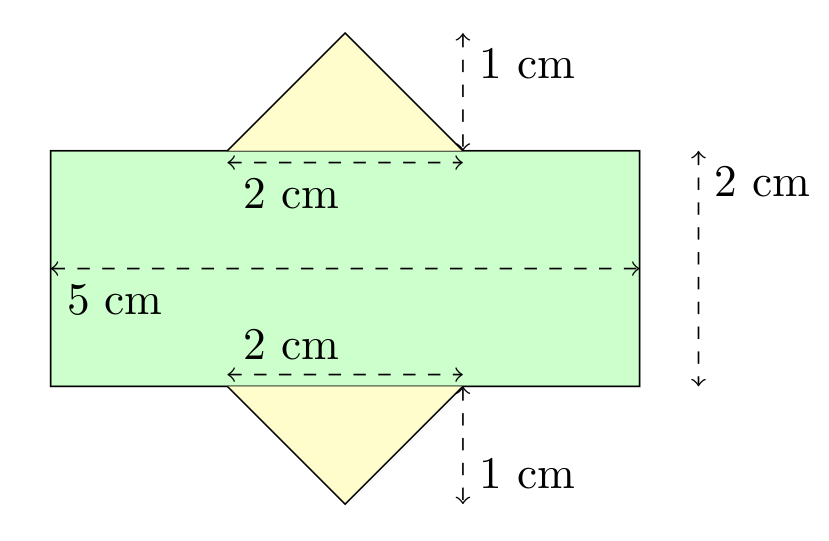
By breaking this composite shape into smaller ones, the area is at hand: $$\begin{align}A_1 &= bh = 5\cdot 2 = 10 \\ A_2 = A_3 &= \frac{bh}{2} = \frac{2\cdot 1}{2} = 1 \\ A_{total} &= A_1+A_2+A_3 = 12\end{align}$$

Unfortunately, this approach can be difficult for a person to use when they cannot physically (or mentally) see the polygon, such as when a polygon is given as a list of many vertices.

Formula

Happily, there is a formula for the area of any simple polygon that only requires knowledge of the coordinates of each vertex. It is as follows: $$A = \sum_{k=0}^{n} \frac{(x_{k+1} + x_k)(y_{k+1}-y_{k})}{2} \tag{1}$$ (Where \({n}\) is the number of vertices, \({(x_k, y_k)}\) is the \({k}\)-th point when labelled in a counter-clockwise manner, and \({(x_{n+1}, y_{n+1}) = (x_0, y_0)}\); that is, the starting vertex is found both at the start and end of the list of vertices.)

It should be noted that the formula is not “symmetric” with respect to the signs of the \({x}\) and \({y}\) coordinates. This can be explained by considering the “negative areas” incurred when adding the signed areas of the triangles with vertices \({(0,0)-(x_k, y_k)-(x_{k+1}, y_{k+1})}\).

In the next sections, I derive this formula using Green’s Theorem, show an example of its use, and provide some applications.

more »