The Möbius function is a rather useful one, especially when dealing with multiplicative functions. But first of all, a few definitions are in order.

Definition 1: Let \(\omega(n)\) be the number of distinct prime divisors of \(n\).

Definition 2: The Möbius function, \(\mu(n)\) is defined as \((-1)^{\omega(n)}\) if \(n\) is square-free and \(0\) otherwise. (A number \(n\) is square-free if there is no prime \(p\) such that \(p^2\) divides \(n\).)

It may be a good idea to compute the following: \(\omega(n)\) and \(\mu(n)\) for \(n=64, 12, 17, 1\) to get an idea of what’s going on.

A Möbius function is an arithmetic function, i.e. a function from \(\mathbb{N}\) to \(\mathbb{C}\). Can you think of some other arithmetic functions?

Definition 3:  If \(f(n)\) is an arithmetic function not identically zero such that \(f(m)f(n)=f(mn)\) for every pair of positive integers \(m, n\) satisfying \((m,n)=1\), then \(f(n)\) is multiplicative.

Theorem 0: \(\mu(n)\) is a multiplicative function.

Proof: The proof is left to the reader.

Theorem 1: If \(f(n)\) is a multiplicative function, so is \(\displaystyle \sum_{d|n} f(d)\).

Before we jump to the proof, let us be clear on the notation. For \(n=12\), \(\displaystyle \sum_{d|n} f(d)=f(1)+f(2)+f(3)+f(4)+f(6)+f(12)\) i.e. the sum taken over the divisors of \(n\).

Proof: Consider the sets \(A= \{d :  0<d, d|n \}\) and \(B= \{d_1d_2 : d_1|m_1, d_2|m_2, (m_1,m_2)=1,m_1m_2=n\}\).

(Note that such \(m_1, m_2\) exist. Take \(m_1=1,m_2=n\)).

Now take \(d \in A\). Then \(1\cdot d\) divides \(1\cdot n\) which means that \(d \in B\) and so \(A \subset B\).

Now take \(s \in B\). So \(s\) is of the form \(d_1d_2\) where \(d_1|m_1\) and \(d_2 |m_2\) such that \((m_1,m_2)=1\) with their product \(n\). So, \(s\) divides \(m\) and hence \(B \subset A\). From these, we infer that \(A=B\).

Now, suppose that \((m,n)=1\). Then \(\displaystyle F(mn)=\sum_{d|mn} f(d)=\sum_{d_1|m,d_2|n,d_1d_2=mn}f(d_1d_2)=\sum_{d_1|m}\sum_{d_2|n} f(d_1d_2)\)

So, $$F(mn)=\sum_{d_1|m}\sum_{d_2|n}f(d_1)f(d_2)(\text{since f is multiplicative})=\sum_{d_1|m}f(d_1)\sum_{d_2|n}f(d_2).$$

Now with this theorem in hand, let us a prove a few more theorems.

 Theorem 2: \(\displaystyle \sum_{d|n} \mu(d)\) is \(0\) if \(n>1\) and \(1\) if \(n=1\).

Proof: The case \(n=1\) is trivial.

Suppose that \(n>1\).

Since \(\mu(n)\) is multiplicative, so is \(\displaystyle F(n)= \sum_{d|n} \mu(d)\). Now let us recall that \(n>1\) can be written as a product of primes, say \(\displaystyle n=p_i^{a_i}\dots p_k^{a_k}\). So, we can write \(F(n)=F(p_1^{a^1})\dots F(p_k^{a_k})\).

As \(a_i\ge 1\), \(F(p_i^{a_i})= 0\) (using the definition of \(\mu\).)That means \(F(n)=0\). The desired conclusion now follows from this discussion.

Before we now move on to a theorem which shows a connection between the Euler’s \(\varphi-\)function and the Möbius function, let us state a really important theorem, also known as the Möbius Inversion formula.

Theorem 3: If \(\displaystyle F(n)=\sum_{d|n}f(d)\) for every positive integer \(n\), then \(\displaystyle  f(n)=\sum_{d|n}\mu(d)F(\frac{n}{d})\).

Proof:  We will flesh this proof in somewhat lesser detail because we have developed most of the techniques related to his proof.

Note that \(\displaystyle \sum_{d|n}\mu(d)F(\frac{n}{d})\)

\(\displaystyle =\sum_{d|n}\mu(d)\sum_{k|(n/d)} f(k)= \sum_{dk|n}\mu(d)f(k)=\sum_{dk|n}\mu(k)f(d)\).

Can the reader now complete the proof? (Hint: Use Theorem 2).

Theorem 4: \(\displaystyle \varphi(n)= n\sum_{d|n} \frac{\mu(d)}{d}.\)

Proof:  To write the proof, we use a lemma.

Lemma: \(\displaystyle \sum_{d|n} \varphi(d)=n\).

Proof of the lemma: Note that for \(n=1\), this is true. Suppose that \(n>1\). Then \(\displaystyle n=p_1^{a_1}\dots p_k^{a_k}\) for some primes \(p_1,\dots, p_k\). As \(\varphi(n)\) is multiplicative, so is \(\displaystyle  F(n)= \sum_{d|n} \varphi(d)\)

That means \(\displaystyle F(n)=\prod_{i=1}^k F(p_i^{a_i})\). A quick calculation reveals that \(F(p_i^{a_i})=p_i^{a_i}\) which gives \(F(n)=n\).

We can now use this lemma and  the Möbius Inversion formula to finish off the proof.

Here as some other problems on multiplicative functions.

Problem 1:  \(\displaystyle \frac{1}{\varphi(n)}=\frac{1}{n}\sum_{d|n}\frac{\mu(d)^2}{\varphi(d)}\).

Problem 2:  For each positive integer \(n\), \(\displaystyle \mu(n)\mu(n+1)\mu(n+2)\mu(n+3) = 0\).

Problem 3: \(\displaystyle \sum_{d|n}|\mu(d)| = 2^{\omega(n)}\).

Introduction

Every so often, the question comes up (either here or elsewhere) of why induction is a valid proof technique. And this is of course a very natural question. Induction is after all rather mysterious compared to the other usual proof techniques. At the same time, it is a very useful one, so it is important that people can be given a satisfactory answer. The question is more precisely “why can we do induction on the natural numbers”, but I am not going to answer that question here. For one thing, the answer depends entirely on how one defines the natural numbers, and for another, induction has nothing to do with the natural numbers. “But wait” you might say. “Did he really just claim that induction has nothing to do with the natural numbers. How can that be? Is induction not something like, we prove something holds for \({0}\) and that if it holds for \({n}\) then it holds for \({n+1}\). How does that even make sense if we are not talking about the natural numbers?” And indeed, the “nothing” was a bit of an overstatement to get your attention. But it turns out that induction is a proof technique that can be used in a much more general setting than that of the natural numbers. This is the viewpoint I will try to explain in detail in this post: Given some set \({X}\), what do we need to be able to use induction to prove that something holds for all elements of \({X}\)?

The usual case

To get started, let us look at the way induction is usually formulated (I will formulate this as a theorem, but as mentioned, I will not give a proof).

Theorem Let \({A\subseteq {\mathbb N}}\) such that \({0\in A}\) and for all \({n\in {\mathbb N}}\) we have \({n\in A\implies n+1\in A}\). Then \({A = {\mathbb N}}\).

At first glance, it seems like this uses some special properties of the natural numbers, namely the facts that we have a \({0}\) and a way to add \({1}\) to any element. But let us look at a different version of induction (often called “strong” induction). Often, we are told that this version is “equivalent” to the usual induction. But as will be seen later, this is either trivial (as both are true statements about the natural numbers), or false (as the theorems do not hold for the same sets when we start to generalize).

Theorem Let \({A\subseteq {\mathbb N}}\) such that for all \({n\in {\mathbb N}}\) we have \({\left(m < n \implies m\in A\right)\implies n\in A}\). Then \({A = {\mathbb N}}\).

(Note that I have the “baseless” version here. But clearly any set satisfying the above will contain \({0}\) since if \({n=0}\) then \({m < n}\) is always false and hence the first implication becomes true regardless of whether \({m\in A}\), which means that the second implication can only be true if \({n\in A}\)). So now we have a version of induction that only uses the ordering of the natural numbers, and this seems like it might be easier to generalize. So let us take a set \({X}\). What sort of ordering must we put on \({X}\) in order to be able to prove that something holds for all \({x\in X}\) by induction? The common answer is “a well-order”, but this is not quite correct, mainly because a well-order is a total order, and it turns out that it is possible to use induction with just a partial order. But let us still start with the more specific question: What sort of total order on \({X}\) allows us to do induction?

Total orders

In this case, the answer is indeed “a well-order”. So let us first look at the definition.

Definition A total order on a non-empty set \({X}\) is called a well-order if any non-empty subset of \({X}\) has a smallest element.

So my claim is that if \({X}\) is a totally ordered set, then we can do induction on \({X}\) if and only if \({X}\) is well-ordered. But this then refers to the “strong” induction. What happened to the other kind? Can we make sense of the other kind if we just have a total order? The answer to the last question is: Almost. If we have a well-ordered set (with a small additional condition), then we can in fact make sense of the usual kind of induction. But it need no longer be a true statement, unless we change some details. Before we move on to the first kind of induction, let us prove the above claim that being well-ordered is both necessary and sufficient. First, we prove that if is sufficient.

Theorem Let \({X}\) be a well-ordered set and \({A\subseteq X}\) be such that for all \({x\in X}\) we have \({\left(y < x \implies y\in A\right)\implies x\in A}\). Then \({A = X}\).

Proof: Let \({B = X\setminus A}\) and assume for the purpose of contradiction that \({B}\) is not empty. Since \({X}\) is well-ordered this means that \({B}\) has a smallest element, call it \({b}\). But now, if \({x\in X}\) with \({x < b}\) then \({x\not\in B}\) since \({b}\) was smallest in \({B}\). Hence for all \({x\in X}\) with \({x < b}\) we have \({x\in A}\), and thus by the assumption on \({A}\), this means that \({b\in A}\) contradicting the choice of \({b}\). \(\Box\)

And then that it is necessary.

Theorem Let \({X}\) be a totally ordered non-empty set such that whenever a subset \({A\subseteq X}\) satisfies \({\left(y < x \implies y\in A\right)\implies x\in A}\) for all \({x\in X}\) then \({A = X}\). Then \({X}\) is well-ordered.

Proof: Let \({B\subseteq X}\) be a subset and assume that \({B}\) does not have a smallest element. Let \({A = X\setminus B}\). We need to show that \({A = X}\) and thus by assumption it is enough to show that if \({x\in X}\) and \({y\in A}\) for all \({y < x}\) then \({x\in A}\). But if \({y\in A}\) for all \({y < x}\) then \({x}\) cannot be in \({B}\), since it would then be the smallest element in \({B}\) (since all strictly smaller elements are not in \({B}\)), and thus \({x\in A}\) as we needed. \(\Box\)

So now the question remains how we can make sense of the first kind of induction, where we needed to have a \({0}\) and needed to be able to add \({1}\) to any element. But there is a very natural way to make sense of these things in a well-ordered set \({X}\), if we just assume one extra thing: \({X}\) does not have a largest element. Namely, we can take \({0}\) to be the smallest element of the set (which exists by assumption). As for adding \({1}\), this really just means “take the next element”, and this makes sense since for any \({x\in X}\) we know that the set \({\{y\in X\mid y > x\}}\) is non-empty (this is where we need \({X}\) to not have a largest element), and thus it has a smallest element, which is the “next” element after \({x}\) (called the immediate successor of \({x}\)). So with these definitions in hand, given a well-ordered set \({X}\) which does not have a largest element, can we do induction on \({X}\)? The answer turns out to be “no”, as the following example demonstrates. The example also illustrates what we need to change to make things work.

Example Let \({X = \{0,1\}\times {\mathbb N}}\) and order \({X}\) lexicographically (so \({(m,n) \leq (m’,n’)}\) if \({m < m’}\) or \({m = m’}\) and \({n\leq n’}\)). It is then easy to check that \({(0,0)}\) is the smallest element of \({X}\) (i.e. we denote \({0 = (0,0)}\)). It is also easy to check that with “\({+1}\)” defined as explained above, we have \({(m,n)+1 = (m,n+1)}\). Let \({A = \{(0,n)\mid n\in {\mathbb N}\}\subseteq X}\). Then the above observations show that \({0\in A}\) and \({a\in A\implies a+1\in A}\) but \({A\neq X}\). But \({X}\) is indeed well-ordered (this is a standard exercise that I leave to the reader), so this is a well-ordered set without a largest element where we cannot use the first kind of induction.

So what is it that goes wrong in the above example? If we look at the usual proof of why induction works for the natural numbers, it is very close to the proof I have presented here that “strong” induction works on any well-ordered set, except that at one point, one will need that if \({n\neq 0}\) then \({n-1}\) makes sense (one considers the complement of the given set, takes the smallest element \({n}\) and notices that this cannot be \({0}\) and then uses the inductive assumption on \({n-1}\)). But how would we define “subtract \({1}\)” in a general well-ordered set? This turns out to not be doable, and this is precisely what goes wrong in the example. More precisely, “subtract \({1}\)” should mean “take the immediate predecessor”, and such need not exist. In the given example, the element \({(1,0)}\) does not have any immediate predecessor, since the elements smaller than \({(1,0)}\) are precisely those in the chosen set \({A}\), and an immediate predecessor would be a largest element in \({S}\), which clearly does not exist. The above suggests how we can remedy the situation: Replace “\({0\in A}\)” by “\({x\in A}\) for any \({x\in X}\) which does not have an immediate predecessor”. And indeed, with this version, we can do induction (I leave the proof as an exercise to the reader. It is just a small change compared to the other proof given).

Partial orders

Back to the more general case: Let \({X}\) be a partially ordered set. What do we need to assume about this partial order in order to do induction on \({X}\) (from now on, by induction I will mean “strong” induction since we cannot really make sense of the other kind in this larger generality). Here the answer turns out to be that we need \({X}\) to be well-founded (actually we do not need an ordering, just any well-founded relation, but I will stick with an ordering). So let us define this.

Definition A partially ordered non-empty set \({X}\) is said to be well-founded if any non-empty subset of \({X}\) has a minimal element.

Let us as previously prove that this condition is both sufficient and necessary to do induction. First, sufficient.

Theorem Let \({X}\) be a well-founded partially ordered set and \({A\subseteq X}\) such that for all \({x\in X}\) we have \({\left(y < x \implies y\in A\right)\implies x\in A}\). Then \({A = X}\).

Proof: Let \({B = X\setminus A}\). Assume for the purpose of contradiction that \({B}\) is not empty, and let \({b\in B}\) be a minimal element. Now it is clear that if \({x\in X}\) with \({x < b}\) then \({x\in A}\) since otherwise \({b}\) would not be minimal. But then \({b\in A}\) contradicting the choice of \({b}\). \(\Box\)

And necessary.

Theorem Let \({X}\) be a partially ordered non-empty set such that whenever a subset \({A\subseteq X}\) satisfies \({\left(y < x \implies y\in A\right)\implies x\in A}\) for all \({x\in X}\) then \({A = X}\). Then \({X}\) is well-founded.

Proof: Let \({B\subseteq X}\) and assume that \({B}\) does not have a minimal element. Let \({A = X\setminus B}\). Now if \({x\in X}\) and \({y\in A}\) for all \({y < x}\) then also \({x\in A}\) as otherwise \({x}\) would be a minimal element of \({B}\). But then by assumption, \({A = X}\) so \({B}\) is empty. \(\Box\)

So now we know when we can do induction. But is this ever useful? And it sure is! For a concrete example of a well-founded set with a non-total order, we can take \({{\mathbb Z}}\) with the ordering \({m\leq n}\) if \({m = n}\) or \({|m| < |n|}\) (the “closer to zero” ordering). Sure, we could also mess a bit with the ordering to make it total, but this makes for a simpler description (for an example where this ordering is used, see my answer here). A useful and easy result for proving that certain sets are well-founded is the following.

Proposition Let \({X}\) be a partially ordered non-empty set such that for all \({x\in X}\), the set \({ \{y\in X\mid y\leq x \} }\) is finite. Then \({X}\) is well-founded.

Proof: Let \({A\subseteq X}\) be a non-empty subset and let \({a\in A}\). Now the set \({ \{x\in X\mid x\leq a \} \cap A}\) is finite and non-empty and thus has a minimal element, which is a minimal element in \({A}\). \(\Box\)

An exercise for the readers

Finally, to end the post, I have an exercise for the readers. Go and find good examples of proofs by induction where the set in question is not the natural numbers. Even better, find ones where the set in question is not the natural numbers, but where the proof ended up being more complicated because the author has taken pains to only do induction on the natural numbers (this need not reflect poorly on the author. If the proof is meant for inexperienced people, then it is often better to give the less direct proof which uses the sort of induction the readers will be familiar with). Go ahead and fill the comments with such examples.

Arguably the first math lesson we’ve had – ever – dealt with counting. Soon, we’re exposed to addition, and later, multiplication. Finally, when we’re fresh into middle school, we take on exponentiation. And every step of the way, we learn that each new operator is shorthand for repeatedly applying the previous one: addition as repeated counting, multiplication as repeated addition, and exponentiation as repeated multiplication. We quickly see that the above operations can be formalized as follows:

• 0. Succession: \( a’ = a + 1\)

• 1. Addition: \(A(a, b) = a + b = \underbrace{a + 1 + 1 + \cdots + 1}_{b \: times} = \underbrace{(a’)’\cdots’}_{b \: times}\)
• 2. Multiplication: \(M(a, b) = a \times b = \underbrace{a + a + a + \cdots + a}_{b \: times}\)
• 3. Exponentiation: \(E(a, b) = a^b = \underbrace{a \times a \times a \cdots \times a}_{b \: times}\)

Several natural questions spring to mind: Can’t we continue this sequence of operators? Can’t another operator be defined as repeated exponentiation, and can’t we repeat that to get a new operator, ad infinitum? The answer is a resounding yes! In fact, the first such an operator already exists and has several applications in various fields: the tetration operator.

Definition:

Tetration is defined as, $$T(a, b) = {}^ba = \underbrace{a^{a^{a^{…^{a}}}}}_{b \> times}$$ As is readily seen, the notation is the exact same as exponentiation, but with the ‘exponent’ to the left. For the sake of this article, we’ll refer to tetration \(n\) times as nth order tetration. That is, if \(b\) in the definition is equal to \(2\), then it is 2nd order tetration, and so on.

Before we go any further, we must specify how to compute values with the tetration operator, as the notation for repeated exponentiation might lead to a certain measure of ambiguity in that regard. For example, given \({}^4 3\), the definition rewrites it as, $$3^{3^{3^3}}.$$ Is this equal to $$((3^3)^3)^3$$ or $$3^{\left[3^{\left(3^3\right)}\right]}?$$ It happens that the second expansion is the correct one, as tetration is defined as right associative, which means it simplifies from the innermost nesting outward. Thus the value of \({}^4 3\) is, $${}^4 3 = 3^{\left[3^{\left(3^3\right)}\right]} = 3^{\left(3^{27}\right)} = 3^{7625597484987}.$$

To put this number into perspective, the above number has approximately \(3.638 \times 10^{12}\) digits, or somewhere over 3 trillion.

Tetration Functions:

In many cases, it is advantageous to define the family of tetration functions so that \(t_n(x) = {}^nx\). The most common functions in this family are \(t_2(x) = {}^2x = x^x\), and \(f_3(x) = {}^3x = x^{x^x}\). Using Wolfram|Alpha, I was able to quickly make two graphs of \(t_2(x)\), shown below:

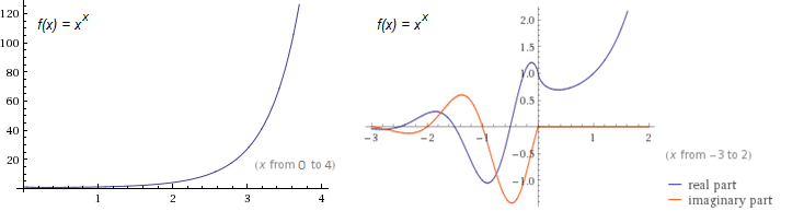
From the first plot, we note just how fast \(t_2(x)\) grows. (Its exponential counterpart, \(f(x) = 2^x\), is only \(16\) at \(x = 4\), whereas \(t_2(x)\) is already \(256\).) From the second, we see the function’s complex behavior for negative \(x\). The only points where \(t_2(x)\) is real for negative values are precisely at the negative integers.

We also note from the second plot how purely real \(t_2(x)\) decreases over a small interval. It is left to the reader as a simple calculus exercise to verify that the real interval where the \(t_2(x)\) decreases is \((0, 1/e)\). It happens that this decreasing behavior occurs for all \(t_n(x)\), where \(n\) is even. A plot of \(t_n(x)\) as \(n \to \infty\) verifies this.

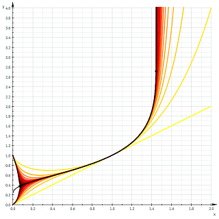
Instantly remarkable from the graph is how half of the functions tend to \(1\) as \(x\) tends to \(0\), and the other half tend to \(0\). In fact, we have, $$\lim_{x \to 0^+} t_n(x) = \begin{cases} 1 & \text{if } n \text{ even} \\ 0 & \text{if } n \text{ odd} \end{cases}$$

Growth of Tetration:

From the previous graphs and calculations it is immediately obvious that tetration outputs very large numbers in exchange for very small ones, on an order even larger than its predecessor, exponentiation.  It seems reasonable to hope that we can prove that its growth rate dominates that of exponentials. Let’s take a look at the following theorem which does just that.

Theorem: for all \(x\) and all \(a > 1, b \geq 2\), we have \(a^x = o({}^bx)\).

Proof: By definition, we have \(a^x = o({}^bx) \Leftrightarrow \lim_{x \to \infty} \frac{a^x}{{}^bx} = 0\). Thus, it suffices to prove the limit for all \(a > 1\) and \(b \geq 2\): With a quick rewrite in terms of exponentials and logarithms, we have, $$\lim_{x \to \infty} \frac{a^x}{{}^bx} = \lim_{x \to \infty} \exp{\left(x\ln{\left(\frac{a}{{}^{b-1}x}\right)}\right)}$$ $$ = \exp{\left(\lim_{x \to \infty}x \lim_{x \to \infty}\ln{\left(\frac{a}{{}^{b-1}x}\right)}\right)}$$ Clearly the first limit is infinity, but the second limit isn’t as obvious. We argue as follows:

Since it is trivial that tetration increases without bound towards infinity, we have \(\lim_{x \to \infty} {}^n x = \infty\). It follows that \(\lim_{x \to \infty} \frac{a}{{}^n x} = \frac{a}{\infty} = 0\), becoming increasingly small and staying positive. We know that \(\ln{(x)} < 0\) in the range \(0 < x < 1\), and so we conclude that \(\lim_{x \to \infty} \ln{(a/{}^{b-1}x)} = -\infty\).

We can now directly compute the limit: $$\exp{\left(\lim_{x \to \infty}x \lim_{x \to \infty}\ln{\left(\frac{a}{{}^{b-1}x}\right)}\right)} = e^{[(\infty) \cdot (-\infty)]} = e^{-\infty} = 0.$$ Q.E.D.

Properties of Tetration:

Unfortunately, tetration defies simple rules such as \(a^b \cdot a^c = a^{b + c}\), but that doesn’t mean that there aren’t any rules at all. What is hard about deriving properties of tetration is that intuition is not able to play a major role, since no one has a ‘feel’ for tetration as they do for exponentiation. If we restrict ourselves to second-order tetration, however, we find several interesting properties, the most important of which I have stated below.

Property 1 (addition rule of tetration):

$${}^2(a + b) = (a + b)^a \cdot (a + b)^b$$

Property 2 (multiplication rule of tetration):

$${}^2(ab) = {}^2a^b \cdot {}^2b^a$$

Property 3 (hyperbolic rule of tetration):

$${}^2x = \sinh{(x \ln{(x)})} + \cosh{(x \ln{(x)})}$$

While theorems 1 and 2 seem reasonable, theorem 3 seems completely out of the blue. In fact, the theorem both relates tetration to the hyperbolic functions and also provides a way of expressing second order tetration without actually using tetration! Below is the derivation:

Proof:

Start with the relation,

$$e^\theta = \sinh{(\theta)} + cosh{(\theta)}$$

Substitute \(\theta = \ln{({}^2x)}\) into the equation and simplify:

$$e^{\ln{({}^2x)}} = \sinh{( \ln{({}^2x)})} + \cosh{(\ln{({}^2x)})}$$

$$ \implies {}^2x = \sinh{(x \ln{(x)})} + \cosh{(x \ln{(x)})}$$

Q.E.D.

To my knowledge, I have never seen any of the above theorems appear in literature on the subject; I derived them myself.

Heading to Arbitrary Bases and Orders:

From the definition of tetration, we see that it can easily be extended to arbitrary bases: \({}^3 0.2\) is easy enough to compute, provided you express it in terms of exponentiation first. The questions, “What is \({}^{-1}2\)? Or \({}^{0.25}6\)?”, however, are not as easy to answer. This question about extending nth order tetration to arbitrary heights, or orders, is the elephant in the room of unsolved questions about this hyper operator. (An analogue of this question would be how to extend factorials to the reals, with the gamma function being the answer.)

Till now, there is no general consensus on tetration’s extension to arbitrary or even negative heights, but there are several competing theories, all with varying levels of difficulty. Perhaps the easiest approach to understand is that of Daniel Geisler, founder of the webpage tetration.org, who attempts to rectify the problem using Taylor series. Another very promising approach given by Kneser much earlier was proven to be both real analytic and unique and works by constructing an Abel function of \(e^x\) and using a Riemann mapping. As the scope of this article is meant to be for undergraduates and/or very bright high school attendees, I shall not discuss the detailed procedures in the constructions but will give links to relevant sources at the end.

Applications:

For many, it is enough to study the properties of tetration simply because of its existence, but for the more applied of the readers among you, it might come as a relief to find out that both tetration and its inverse (and variants thereof) find application in many areas, with other fields also being candidates for its use.

Starting from mathematics itself, one finds that the modern version of the Ackermann function is actually equal to base-two nth order tetration, and can thus help in easily expressing the outputs of such a function. We have,

$${}^n2 = A(4, n-3) + 3.$$

(Note: This \(A(a, b)\) is the Ackermann function, and not the “addition” function given at the beginning of the article, even though they both are denoted \(A\).)

The original three-argument version of Ackermann’s function gives rise to tetration more generally:

$$φ(a, b, 3) = {}^ba.$$

Note that the Ackermann function is discrete, so finding a continuous version of the function is equivalent to extending tetration to all heights.

Another application is in computing the number of elements in the Von Neumann universe construction in set theory: the number is \({}^2n\), where here \(n\) is the stage of the construction. It serves as an aid in understanding the rapid growth of the elements in each stage.

If one considers the inverse function of second order tetration, called the super square root \(\text{ssrt(}x\text{)}\), we find several other applications, mentioned below.

Define $$\text{wzl(}x\text{)} = \text{ssrt(}10^x\text{)}$$ This function is called the ‘wexzal’ (a modification of the German word for ‘root’), and was coined and studied extensively in the self-titled paper, found below. According to the paper, using plotting software and extensive numerical tables for comparison, the authors found a more accurate equation for modeling velocity decay in ballistics which is the equation, $$v = \frac{a}{\text{wzl(}e^{bx}\text{)}}$$ as apposed to the traditional equation, $$v = \frac{a}{e^{bx}}.$$ Note that \(a\) and \(b\) are parameters depending on each case. This new equation also has the advantage of being integrable to find the flight time, so nothing is lost from the less accurate equation’s advantages.

Similarly, we can find using this variation of tetration’s inverse significantly better fits for various firearm quantities such as muzzle velocity as well as for motor vehicle acceleration.

Conclusion

So what’s the whole point of this? This article serves as a reminder that there are many areas of mathematics left untouched despite the vast compendium we have now. It simply examines one such unturned rock and gives a look into possible developments into the theory of hyper operators. Regrettably, some topics were not discussed for the sake of brevity, such as tetration’s inverse operation and calculus with the tetration function. For the eager reader, though, I have included some resources to further knowledge on the subject.

Further Reading and References

• Wexzal paper, discussing quite thoroughly the tetration function and its inverse as well as the wexzal function and its applications.
• Daniel Geisler’s site on tetration and his proposed extension.
• The tetration forum, which hosts mostly higher-level math discussions on tetration and related concepts.
• Kneser’s analytic extension procedure of tetration and its inverse and a proof of its uniqueness
• My own brief research on the properties of second-order tetration.

Dealing With Risk

Consider a small company which uses a million dollar machine as an essential part of its operations. Suppose that there is a 10% chance that the machine will break down and need replacement in a given year. If the machine breaks down and the company replaces it, they can continue their operations for the rest of the year. If they machine breaks down and the company is unable to pay for a replacement, the company will have to cease its operations permanently. What is the probability that the company will have to cease its operations permanently?

To be fair, this is not really a question about mathematics. It is a question about business and risk. A business must find a strategy that minimizes its costs and maximizes its income, even in the face of uncertainty. Of course, the company will receive no income if its machine breaks down. So the company must balance the possibility of a break down with the certain costs to protect itself from a break down.

A Particularly Ineffective Strategy

The company might have heard of the expected value principle, an axiom of actuarial science that tells us the economic value of a random variable amount of money is the expectation of the variable, and decide to put $100,000 in a savings account to protect against the loss of the machine. This strategy is too naive. Obviously, the $100,000 isn’t going to pay for a replacement machine when the old one breaks down. So in any given year, the company faces a 10% chance of having to cease its operations.  Worse yet, since the money the company saved offers no protection, it was used non-productively.

A Slightly Better Strategy

The company might have realized that, as stated, the number of years until the machine has its first break down is a geometric random variable \(N\), whose probability mass function is given by:

$$ \newcommand{\P}[1]{\mathbf{P}\!\left[#1\right]} \P{N = n} = (1 – p)^{n-1} p, $$

where, in this case, \(p = 10\%\).

The company might decide to save $100,000 at the start of every year, until they have saved enough money to replace the machine. Observe that the company will not have saved enough money until the 10th year. That is to say, they will face a 10% risk of having to cease operations permanently, every year, for the first nine years of operation. After that, they will have a 0% risk of having to cease operations. Since \(N\), the number of years until the first break down, has a known probability distribution, we can compute

$$ \begin{align} \P{N \leq 9} &= 1 – (1 – p)^9 \\ &= 1 – 0.9^9 \\ &\approx 0.613 \end{align} $$

That is to say, there is approximately a 61.3% chance that the first break down will occur in the first nine years of operation, which would put the company out of business.

This strategy is wasteful even if the company manages to beat the odds. By the tenth year, the company will have saved up a million dollars which could be put to use productively.

How Insurance Works

At its most fundamental level, insurance is a system for reducing the adverse effects of random events. Insurance does not eliminate risks, but it transfers the financial burden of a loss to an insurance company, in exchange for a certain sequence of payments from the customer. By pooling together a large number of these risks, an insurance company is able to increase the “predictability” of its losses. Analyzing the process by which pooling works essentially requires a central limit theorem, which tells us that the sum of large numbers of random variables (with finite variance) converges in distribution to a normal random variable. By modelling its pool in this way, an insurance company is able to budget for losses much more efficiently than any one of its consumers could by themselves.

So, let’s suppose that there are 1000 small companies in the pool, and each face the same risk of a breakdown, with the same distribution of losses. Then the total expected losses are one hundred million, since we expect that 10% of the machines will break down. Using the central limit theorem, we see that the losses the insurance company will face are approximately normally distributed, with a mean of one hundred million, and a standard deviation of about 9.5 million dollars.

This means that if the insurance company collects approximately 109.5 million dollars in premiums in a year, then there is about a 84% chance that they will be able to pay for every loss that year. If they collect approximately 119 million dollars in premiums, then there is about a 97.6% chance that they can pay for every loss that year. If they collect approximately 128 million dollars in premiums, there is more than a 99% chance that they can pay for every loss.

Calculating the risk each individual company now faces is involved, but we can make some observations. For a company to close in the current year:

• its machine would have to break down
• at least 128 other machines would have to break down before before it

It is clear that the latter event will be rare, especially when compared to the risk the company originally faced in a year.  Indeed, we will demonstrate that the probability that any one company closes is less than 1%.

We will do this by using the law of total probability. Let \(F\) be the event that the company fails.  Then

$$ \begin{align} \P{F} &= \P{F|N \leq 128}\P{N\leq 128} + \P{F|N > 128}\P{N> 128} \\ &= 0\cdot \P{N\leq 128} + \P{F|N > 128}\P{N > 128}\\ &= \P{F|N > 128}\P{N > 128}\\ \end{align} $$

Notice that the argument so far agrees with the observations made above. In fact, it was informed by the observations.

Now we must compute \(\P{F|N > 128}\P{N > 128}\). This is not straight-forward, and in fact, we do not have enough information to do it without making additional assumptions. The issue is that we do not have any idea how failures are distributed in time. For example, it seems intuitively plausible that a machine in a factory with poor maintenance would fail before a machine in a factory with good maintenance.

We will assume that if there are \(N\) break downs, all \(N!\) orders in which they can occur are equally likely. We can make some observations. First, 128 out of \(N\) companies will get paid. The rest are out of luck. In particular, the probability that our company gets paid is \(\frac{128}{N}\). The probability that our company doesn’t get paid is \(\frac{N – 128}{N}\).

So, using the law of total probability again, we compute:

$$ \begin{align} \P{F|N > 128}\P{N > 128} &= \sum_{n=128}^\infty \P{F|N = n}\P{N = n} \\ &= \sum_{n=128}^\infty \frac{n – 128}{n} f_N(n) \\ &= \sum_{n=128}^\infty \frac{n – 128}{n} F_N(n) – F_N(n+1) \end{align} $$

which is approximately equal to 0.00003915. Again, this number represents the approximate probability that any given company will fail because its machine breaks down in any given year. This is a vast improvement over the situation where there was a 10% chance of failure. To put it in perspective, the distribution of the number of years until the company fails is geometric, with \(p = 0.00003915\), so that the average number of years until a specific company fails is 25.5 thousand years.

This sort of insurance represents a benefit to society in a variety of ways. Insurance lowers the amount of money a business has to raise to protect itself from failure. And so insurance frees capital for more productive purposes.

This model presents property insurance at its most basic level. Real insurance companies have operating costs, and have to follow federal and state regulations for how much they collect in premiums and how they manage the pool of risk. Real policies might have deductibles and other stipulations to fine-tune the amount of risk that gets transferred. Real insurance customers have preferences about how they want to spend their money. The insurance business is what happens when these complex factors meet the basic risk transfer model. An actuary’s job is to understand this basic model and all the fiddly exceptions, laws, and business practices in order to make insurance companies possible and profitable.

Where to find out more:

An actuary must achieve mastery of several topics, including basic and intermediate probability and statistics. If you want to learn more, check out Be An Actuary or talk to a math, business, or finance professor.

Adapted with permission from Poisson Labs.

There are some questions that are really easily posed, have an obvious answer, but are in fact really, really hard to answer in a mathematically satisfactory way. Two examples are:

1. How many holes does a doughnut have?
2. Are a ball and a disk “the same thing”? Meaning: can I deform the first to make it the second in a way that locally preserves its structure, i.e. without tearing, and without “squishing” things too much?

The intuitive (and actually correct) answers are: one, and no. However, in order to prove them true, we’ll have first to formalize the questions in mathematical language, and then to develop a theory that will allow us to work on them.

Let’s start with the first question. “A doughnut” can be interpreted in two ways: it could be a filled doughnut, that is the space \(S^1\times D^2\), where \(S^1\) denotes the circle, and \(D^2\) the \(2\)-dimensional disc , or it could be a hollow doughnut, corresponding to the torus \(T^2=S^1\times S^1\). Both of them are examples of topological spaces, so we will generalize the question to: given a topological space \(X\), how many holes does \(X\) have? If you don’t know what a topological space is, just take \(X\) to be one of the examples of doughnuts given above, unless otherwise specified.

The next question we have to answer is: what is a hole? We have many different examples of things we would like to consider holes. One is our hole in the doughnut, but we could also take the space, \(\mathbb{R}^3\), and take away a ball from it, or a infinitely long filled cylinder. Notice that the last two examples are fundamentally different, in the following way: if we take away an infinite cylinder from the space and draw a closed curve around it, we will never be able to deform it to a path not containing the cylinder, or to a single point, without “breaking” it, while we deform every closed curve to a single point in the very last example. However, if we were to put a sphere around the ball we removed in the last example, then we could not deform it to a point, while we could do it for every sphere in our space without a cylinder.

Noticing that a closed path looks very much like a circle, we can use this to distinguish between various kinds of holes. We will informally call an \(n\)-dimensional hole an \(n\)-sphere \(S^n\) that cannot be deformed to a single point without tearing it, where we define: $$S^n=\left\{x\in\mathbb{R}^{n+1}:\lvert x\rvert^2=1\right\}$$ Notice that \(S^1\) is the circle, and \(S^2\) is the sphere. Now, spheres look like really simple spaces, but are in fact quite difficult to work with. However, there’s something we can do to avoid working directly with spheres while keeping intact the essence of what we have said until now: we can cut up spheres in smaller “triangular” pieces. We make the following definition:

Definition: Let \(v_0,\ldots,v_n\in\mathbb{R}^{m}\), where \(m\ge n\). We define the affine \(n\)-dimensional singular simplex \([v_0,\ldots,v_n]\) as the closed convex hull of the points \(v_0,\ldots,v_n\), that is: $$[v_0,\ldots,v_n]=\left\{\sum_{k=0}^nt_kv_k:t_k\in[0,1]\forall k,\ \sum_{k=0}^nt_k=1\right\}$$ We also define the standard \(n\)-simplex as \(\Delta^n=[e_0,\ldots,e_n]\subset\mathbb{R}^{n+1}\), where \(e_i\in\mathbb{R}^{n+1}\) are the standard basis elements.

Notice that the standard \(2\)-simplex is in fact a triangle, and the standard \(3\)-simplex is a tetrahedron. So this definition gives a sensible generalization of what a triangle of dimension \(n\) should be. Let’s now cover the circle \(S^1\) with \(1\)-simplices, and the sphere \(S^2\) with \(2\)-simplices. We immediately notice that they have something special with respect to a random collection of simplices: they have no boundary, that is, the triangles composing them have the sides glued together in such a way that they cancel each other. This leads us to make the next definition:

Definition: The \(i\)-th face of an \(n\)-simplex \(a=[v_0,\ldots,v_n]\) is the \((n-1)\)-simplex \(a^{(i)}[v_0,\ldots,v_{i-1},v_{i+1},\ldots,v_n]\). The boundary of the simplex is the (formal) sum of \((n-1)\)-simplices: $$ \partial a=\sum_{k=0}^n(-1)^ka^{(k)}$$

Notice that the boundary of a simplex is a sum of simplices of lower dimension, so we would like to define some set of simplices where we are allowed to take sums in a sensible way. Also, we would like our simplices to live in our topological space \(X\), and not only in \(\mathbb{R}^m\). So we define the group of \(n\)-simplices in \(X\), denoted by \(S_n(X)\), as the free abelian group generated by continuous maps \(\sigma:\Delta^n\to X\). This simply means that the object (called chains) of \(S_n(x)\) are finite sums of simplices of dimension \(n\) in \(X\) (this is why we take maps from the standard simplex to \(X\)), and that we can sum two such objects in the obvious way, for example if we have two chains \(\sigma_1\) and \(\sigma_2\), then we have: $$(2\sigma_1+\sigma_2)+3\sigma_2=2\sigma_1+4\sigma_3$$ The boundary defines then a map (in fact, a group homomorphism) from \(S_n(x)\) to \(S_{n-1}(X)\), defined on the generators \(\sigma:\Delta^n\mapsto X\) as: $$\partial \sigma=\sum_{k=0}^n(-1)^k\sigma^{(k)}$$ where \(\sigma^{(k)}\) is simply the map \(\sigma\) restricted to the \(i\)-th face of \(\Delta^n\). The sequence of groups \(S_n(X)\) together with the boundary maps defines a sequence: $$\ldots\stackrel{\partial_{n+1}}{\longrightarrow} S_n(X)\stackrel{\partial_{n}}{\longrightarrow} S_{n-1}(x)\stackrel{\partial_{n-1}}{\longrightarrow}\ldots\stackrel{\partial_{2}}{\longrightarrow} S_1(X)\stackrel{\partial_{1}}{\longrightarrow} S_0(X)\to 0$$ where the composition of two consecutive arrows gives the zero map (this can be easily checked by writing down what happens to a generator and rearranging a couple of sums). This kind of sequence is really important in some areas of mathematics, and they have a special name: they are called chain complexes. As we have seen, of all the elements in the chain complex we want to consider those with no boundary, that is, elements in: $$Z_n=\ker(\partial_n)=\{c\in S_n(X)|\partial c=0\}\subseteq S_n(X)$$ We call these elements cycles. They represent in some sense “closed things”, like circles, spheres, but also for example tori (i.e. our hollow donuts) and similar stuff. Moreover, we would like to identify two cycles whenever they represent, for example, two closed paths that can be deformed in such a way that the first becomes equal to the second. Notice that if this is the case, then during the deformation the first curve will draw some kind of annulus, which we can cover with \(2\)-simplices and (as a chain) will have as boundary the first path minus the second one. This leads us to the idea of identifying two cycles whenever their difference is a boundary. Thus we define the homology groups of \(X\) by: $$H_n(X)=Z_n/B_n$$ where \(B_n=\partial_{n+1}(S_{n+1}(X))\) is the set of boundaries.

These groups have a great deal of nice properties. First of all, they are topological invariants. This means that if two spaces are “essentially the same” (the technical term is homeomorphic, meaning that there exist a continuous bijection with continuous inverse between the two), then their homology groups are equal. Another similar thing is that if \(Y\) is a subspace of \(X\), and we can deform \(X\) to \(Y\) without deforming \(Y\), then \(X\) and \(Y\) have the same homology groups. The other useful properties are mostly too technical to be stated here without making this post excessively long. Also, unfortunately, we don’t have enough tools to compute the homology groups of spaces more complicated than, say, finite unions of points, or balls, or \(\mathbb{R}^n\). So when needed I will just state the results, and if you are interested in the computations, you can try to consult one of the bibliographical references I will give at the end.

Whew! We’ve come a long way from the original question of counting the number of holes in a doughnut! But finally we can answer the question. From our definitions, the \(n\)-th homology group should more or less count the number of \(n\)-dimensional holes in the space. For example, for the filled doughnut we have: $$H_n(S^1\times D^2)=\begin{cases} \mathbb{Z}&\text{for $ n=0,2$} \\ 0 &\text{else } \end{cases}$$ The \(0\)-th group doesn’t really matters to us, in fact all it does is to count the number of “pieces” of which our space is made of. The \(1\)-st homology group, however, gives us the information we needed: up to equivalence, there is exactly one \(1\)-chain which is not a boundary (we get \(\mathbb{Z}\) because we can also count twice the same chain, or three times, etc.). This means that there is one circle (or something analogous) that cannot be deformed to be a point, and thus that there is exactly one \(1\)-dimensional hole. Similarly, for the hollow doughnut we have: $$H_n(S^1\times S^1)=\begin{cases} \mathbb{Z} &\text{for $n=0,2$}\\ \mathbb{Z}^2 &\text{for $n=1$}\\ 0 &\text{else}\end{cases}$$

Thus we have one \(2\)-dimensional hole (the whole hollow part of the doughnut), and two \(1\)-dimensional holes (the circle going around the central hole of the doughnut, and the circle going around the hole formed by the hollow part).

As a bonus, we can also use homology to answer our second question. As I have stated, two homeomorphic spaces (“essentially the same”, remember?) have the same homology groups. Now if a ball \(B^3\) in space were homeomorphic to a disk \(B^2\), then removing exactly one interior point in each of those spaces in a sensible way we would again get homeomorphic spaces. However a ball without a point deforms nicely to a sphere, and a disk without a point to a circle, and we have: \begin{gather}H_n(S^1)=\begin{cases}\mathbb{Z} &\text{if $n=0,1$}\\ 0 &\text{else}\end{cases},\\ H_n(S^2)=\begin{cases} \mathbb{Z} &\text{if $n=0,2$}\\ 0 &\text{else} \end{cases}\end{gather}

which is exactly what we would expect from our intuition about \(n\)-dimensional holes. Since these are not equal, the two spaces cannot be homeomorphic, and thus we are done.

Those two problems we just solved are two of the many applications of homology theory, and indeed of the larger framework, which is called algebraic topology. If you want to know more on the subject, here are three books you can try to read:

• Allen Hatcher, Algebraic Topology
• Glen E. Bredon, Topology and Geometry
• Edwin H. Spanier, Algebraic Topology

Matching theory is an active field in mathematics, economics, and computer science. It ensured a [Nobel memorial prize][1] for [Alvin E. Roth][2] and [Lloyd S. Shapley][3] in 2012. The theory is applied in the real world to match students and colleges, doctors and hospitals, and to organize the allocation of donor organs. It all started with a beautiful paper by [David Gale][4] and Lloyd Shapley in 1962: [College Admissions and the Stability of Marriage][5] (read it!). In this post, we study the simplest version of what is known as the stable marriage problem and take a look at inherent conflicts. The exposition follows chapter 22 of the wonderful book [Game Theory][6] by Michael Maschler, Eilon Solan, and Shmuel Zamir.

What are stable matchings?

There is a set \( G \) of \( n \) girls and a set \( B \) of \( n \) boys. All girls and boys are heterosexual and desperate enough to prefer every member of the opposite sex to staying single. Each girl \( g \) has preferences over the boys, represented by a [total order][7] \( \succeq_g \) on \( B \). Similarly, each boy \( b \) has preferences over the girls, represented by a total order \(\succeq_b\) on \( G \).

We want to pair up the girls and the boys. Formally, a matching is simply a [bijection][8] \( M \) from \(G\) to \(B\) and if \( f(g)=b \), we say that \( g \) and \( b \) are matched (under \( M\)). Now, nobody can force the girls and boys to be together, so we have to look at matchings in which the boys and girls are relatively content with whom they get. To be precise, a matching is stable if we cannot find a girl and a boy who prefer each other under their preference ordering to whomever they are matched with.

Are there any?

Before we go into a deep study of stable matchings, we ought to make sure that there are stable matchings. We do so by giving an explicit algorithm for finding a stable matching, the boy courtship algorithm.

more »

I wrote an article with Irving Kaplansky on indefinite binary quadratic forms, integral coefficients. At the time, I believe I used high-precision continued fractions or similar. It took me years to realize that the right way to solve Pell’s equation, or find out the “minimum” of an indefinite form (and other small primitively represented values), or the period of its continued fraction, was the method of “reduced” forms in cycles/chains, due to Lagrange, Legendre, Gauss. It is also the cheapest way to find the class number and group multiplication for ideals in real quadratic fields, this probably due to Dirichlet. For imaginary quadratic fields, we have easier “reduced” positive forms.

A binary quadratic form, with integer coefficients, is some $$ f(x,y) = A x^2 + B xy + C y^2. $$ The discriminant is $$ \Delta = B^2 – 4 A C. $$ We will abbreviate this by $$ \langle A,B,C \rangle. $$ It is primitive if \({\gcd(A,B,C)=1. }\) Standard fact, hard to discover but easy to check: $$ (A x^2 + B x y + C D y^2 ) (C z^2 + B z w + A D w^2 ) = A C X^2 + B X Y + D Y^2,$$ where \({ X = x z – D yw, \; Y = A xw + C yz + B yw. }\) This gives us Dirichlet’s definition of “composition” of quadratic forms of the same discriminant, $$ \langle A,B,CD \rangle \circ \langle C,B,AD \rangle = \langle AC,B,D \rangle. $$ In particular, if this \({D=1,}\) the result represents \({1}\) and is (\({SL_2 \mathbb Z}\)) equivalent to the “principal” form for this discriminant. Oh, duplication or squaring in the group; if \({\gcd(A,B)=1,}\) $$ \langle A,B,AD \rangle^2 = \langle A^2,B,D \rangle. $$ This comes up with positive forms: \({ \langle A,B,C \rangle \circ \langle A,-B,C \rangle = \langle 1,B,AC \rangle }\) is principal, the group identity. Probably should display some \({SL_2 \mathbb Z}\) equivalence rules, these are how we calculate when things are not quite right for Dirichlet’s rule: $$ \langle A,B,C \rangle \cong \langle C,-B,A \rangle, $$ $$ \langle A,B,C \rangle \cong \langle A, B + 2 A, A + B +C \rangle, $$ $$ \langle A,B,C \rangle \cong \langle A, B – 2 A, A – B +C \rangle. $$

more »

In this post I describe how simple facts about polynomials are applied in correcting errors, for example scratches on compact disks.  The same technique is used in many other places, e.g. in the 2-dimensional QuickResponse  bar codes.

Elements

The two facts from algebra that we need are:

Theorem 1. A polynomial of degree \(n\) has at most \(n\) zeros.

Theorem 2. If \((x_1,y_1),(x_2,y_2),\ldots,(x_n,y_n)\) are \(n\) points on the \(xy\)-plane such that \(x_i\neq x_j\) whenever \(i\neq j\), then there is a unique polynomial \(f(x)\) of degree \(<n\) such that \(f(x_i)=y_i\) for all \(i\).

So, if \(n=2\), we want the polynomial \(f(x)\) to be linear. In that case, the graph \(y=f(x)\) will be the line passing through the points \((x_1,y_1)\) and \((x_2,y_2)\). Similarly, when \(n=3\) we want the polynomial to be (at most) quadratic, and we want its graph to pass through the given three points. Finding the coefficients of such a quadratic is not too arduous an exercise in linear systems of equations. For general \(n\) there is a known formula for the polynomial \(f(x)\) called Lagrange’s interpolation polynomial . The uniqueness of such a polynomial follows from Theorem 1. If \(f_1(x)\) and \(f_2(x)\) were two different polynomials of degree \(<n\) passing through all these \(n\) points, then their difference \(f_1(x)-f_2(x)\) is also of degree \(<n\) and vanishes at all the points \(x_i, i=1,2,\ldots,n\), which is impossible by Theorem 1.

Extending a message using a polynomial

The applications I discuss are about communication. We have two parties, a transmitter and a receiver. The transmitter wants to send a message to the receiver. We assume that they have in advance agreed upon a method of coding the messages to sequences of numbers \(y_1,y_2,\ldots,y_k\) for some natural number \(k\). The simplest way of communicating would be for the transmitter to simply write this list of numbers to a channel that the receiver can later read. The channel could be something like a note that you pass to a classmate or it could be compact disk, where the transmitter just writes the numbers. It could be something fancier like a radio frequency band, or an optical fiber, but we ignore the physical nature of the channel here.

more »

A common method used to find the area of a polygon is to break the polygon into smaller shapes of known area. For example, one can separate the polygon below into two triangles and a rectangle:

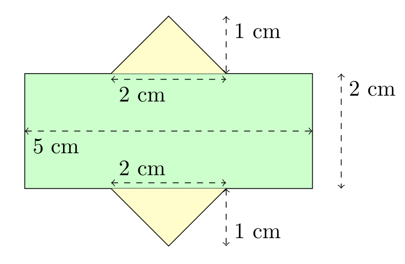
By breaking this composite shape into smaller ones, the area is at hand: $$\begin{align}A_1 &= bh = 5\cdot 2 = 10 \\ A_2 = A_3 &= \frac{bh}{2} = \frac{2\cdot 1}{2} = 1 \\ A_{total} &= A_1+A_2+A_3 = 12\end{align}$$

Unfortunately, this approach can be difficult for a person to use when they cannot physically (or mentally) see the polygon, such as when a polygon is given as a list of many vertices.

Formula

Happily, there is a formula for the area of any simple polygon that only requires knowledge of the coordinates of each vertex. It is as follows: $$A = \sum_{k=0}^{n} \frac{(x_{k+1} + x_k)(y_{k+1}-y_{k})}{2} \tag{1}$$ (Where \({n}\) is the number of vertices, \({(x_k, y_k)}\) is the \({k}\)-th point when labelled in a counter-clockwise manner, and \({(x_{n+1}, y_{n+1}) = (x_0, y_0)}\); that is, the starting vertex is found both at the start and end of the list of vertices.)

It should be noted that the formula is not “symmetric” with respect to the signs of the \({x}\) and \({y}\) coordinates. This can be explained by considering the “negative areas” incurred when adding the signed areas of the triangles with vertices \({(0,0)-(x_k, y_k)-(x_{k+1}, y_{k+1})}\).

In the next sections, I derive this formula using Green’s Theorem, show an example of its use, and provide some applications.

more »