(or How I implemented an unanswered question tracker and began to grasp the size of the site.)

I’m not sure when it happened, but Math.StackExchange is huge. I remember a distant time when you could, if you really wanted to, read all the traffic on the site. I wouldn’t recommend trying that anymore.

I didn’t realize just how vast MSE had become until I revisited a chatroom dedicated to answering old, unanswered questions, The Crusade of Answers. The users there especially like finding old, secretly answered questions that are still on the unanswered queue — either because the answers were never upvoted, or because the answer occurred in the comments. Why do they do this? You’d have to ask them.

But I think they might do it to reduce clutter.

Sometimes, I want to write a good answer to a good question (usually as a thesis-writing deterrence strategy).

And when I want to write a good answer to a good question, I often turn to the unanswered queue. Writing good answers to already-well-answered questions is, well, duplicated effort. [Worse is writing a good answer to a duplicate question, which is really duplicated effort. The worst is when the older version has the same, maybe an even better answer]. The front page passes by so quickly and so much is answered by really fast gunslingers. But the unanswered queue doesn’t have that problem, and might even lead to me learning something along the way.

In this way, reducing clutter might help Optimize for Pearls, not Sand. [As an aside, having a reasonable, hackable math search engine would also help. It would be downright amazing]

And so I found myself back in The Crusade of Answers chat, reading others’ progress on answering and eliminating the unanswered queue. I thought to myself How many unanswered questions are asked each day? So I wrote a script that updates and ultimately feeds The Crusade of Answers with the number of unanswered questions that day, and the change from the previous day at around 6pm Eastern US time each day.

I had no idea that 166 more questions were asked than answered on a given day. There are only four sites on the StackExchange network that get 166 questions per day (SO, MathSE, AskUbuntu, and SU, in order from big to small). Just how big are we getting? The rest of this post is all about trying to understand some of our growth through statistics and pretty pictures. See everything else below the fold.

more »

While teaching a largely student-discovery style elementary number theory course to high schoolers at the Summer@Brown program, we were looking for instructive but interesting problems to challenge our students. By we, I mean Alex Walker, my academic little brother, and me, David Lowry-Duda. After a bit of experimentation with generators and orders, we stumbled across a proof of Wilson’s Theorem, different than the standard proof.

Wilson’s theorem is a classic result of elementary number theory, and is used in some elementary texts to prove Fermat’s Little Theorem, or to introduce primality testing algorithms that give no hint of the factorization.

Theorem 1 (Wilson’s Theorem) For a prime number \({p}\), we have $$ (p-1)! \equiv -1 \pmod p. \tag{1}$$

The theorem is clear for \({p = 2}\), so we only consider proofs for “odd primes \({p}\).”

The standard proof of Wilson’s Theorem included in almost every elementary number theory text starts with the factorial \({(p-1)!}\), the product of all the units mod \({p}\). Then as the only elements which are their own inverses are \({\pm 1}\) (as \({x^2 \equiv 1 \pmod p \iff p \mid (x^2 – 1) \iff p\mid x+1}\) or \({p \mid x-1}\)), every element in the factorial multiples with its inverse to give \({1}\), except for \({-1}\). Thus \({(p-1)! \equiv -1 \pmod p.} \diamondsuit\)

Now we present a different proof.

Take a primitive root \({g}\) of the unit group \({(\mathbb{Z}/p\mathbb{Z})^\times}\), so that each number \({1, \ldots, p-1}\) appears exactly once in \({g, g^2, \ldots, g^{p-1}}\). Recalling that \({1 + 2 + \ldots + n = \frac{n(n+1)}{2}}\) (a great example of classical pattern recognition in an elementary number theory class), we see that multiplying these together gives \({(p-1)!}\) on the one hand, and \({g^{(p-1)p/2}}\) on the other.

As \({g^{(p-1)/2}}\) is a solution to \({x^2 \equiv 1 \pmod p}\), and it is not \({1}\) since \({g}\) is a generator and thus has order \({p-1}\). So \({g^{(p-1)/2} \equiv -1 \pmod p}\), and raising \({-1}\) to an odd power yields \({-1}\), completing the proof \(\diamondsuit\).

After posting this, we have since seen that this proof is suggested in a problem in Ireland and Rosen’s extremely good number theory book. But it was pleasant to see it come up naturally, and it’s nice to suggest to our students that you can stumble across proofs.

It may be interesting to question why \({x^2 \equiv 1 \pmod p \iff x \equiv \pm 1 \pmod p}\) appears in a fundamental way in both proofs.

This post appears on the author’s personal website davidlowryduda.com and on the Math.Stackexchange Community Blog math.blogoverflow.com.

There are some questions that are really easily posed, have an obvious answer, but are in fact really, really hard to answer in a mathematically satisfactory way. Two examples are:

1. How many holes does a doughnut have?
2. Are a ball and a disk “the same thing”? Meaning: can I deform the first to make it the second in a way that locally preserves its structure, i.e. without tearing, and without “squishing” things too much?

The intuitive (and actually correct) answers are: one, and no. However, in order to prove them true, we’ll have first to formalize the questions in mathematical language, and then to develop a theory that will allow us to work on them.

Let’s start with the first question. “A doughnut” can be interpreted in two ways: it could be a filled doughnut, that is the space \(S^1\times D^2\), where \(S^1\) denotes the circle, and \(D^2\) the \(2\)-dimensional disc , or it could be a hollow doughnut, corresponding to the torus \(T^2=S^1\times S^1\). Both of them are examples of topological spaces, so we will generalize the question to: given a topological space \(X\), how many holes does \(X\) have? If you don’t know what a topological space is, just take \(X\) to be one of the examples of doughnuts given above, unless otherwise specified.

The next question we have to answer is: what is a hole? We have many different examples of things we would like to consider holes. One is our hole in the doughnut, but we could also take the space, \(\mathbb{R}^3\), and take away a ball from it, or a infinitely long filled cylinder. Notice that the last two examples are fundamentally different, in the following way: if we take away an infinite cylinder from the space and draw a closed curve around it, we will never be able to deform it to a path not containing the cylinder, or to a single point, without “breaking” it, while we deform every closed curve to a single point in the very last example. However, if we were to put a sphere around the ball we removed in the last example, then we could not deform it to a point, while we could do it for every sphere in our space without a cylinder.

Noticing that a closed path looks very much like a circle, we can use this to distinguish between various kinds of holes. We will informally call an \(n\)-dimensional hole an \(n\)-sphere \(S^n\) that cannot be deformed to a single point without tearing it, where we define: $$S^n=\left\{x\in\mathbb{R}^{n+1}:\lvert x\rvert^2=1\right\}$$ Notice that \(S^1\) is the circle, and \(S^2\) is the sphere. Now, spheres look like really simple spaces, but are in fact quite difficult to work with. However, there’s something we can do to avoid working directly with spheres while keeping intact the essence of what we have said until now: we can cut up spheres in smaller “triangular” pieces. We make the following definition:

Definition: Let \(v_0,\ldots,v_n\in\mathbb{R}^{m}\), where \(m\ge n\). We define the affine \(n\)-dimensional singular simplex \([v_0,\ldots,v_n]\) as the closed convex hull of the points \(v_0,\ldots,v_n\), that is: $$[v_0,\ldots,v_n]=\left\{\sum_{k=0}^nt_kv_k:t_k\in[0,1]\forall k,\ \sum_{k=0}^nt_k=1\right\}$$ We also define the standard \(n\)-simplex as \(\Delta^n=[e_0,\ldots,e_n]\subset\mathbb{R}^{n+1}\), where \(e_i\in\mathbb{R}^{n+1}\) are the standard basis elements.

Notice that the standard \(2\)-simplex is in fact a triangle, and the standard \(3\)-simplex is a tetrahedron. So this definition gives a sensible generalization of what a triangle of dimension \(n\) should be. Let’s now cover the circle \(S^1\) with \(1\)-simplices, and the sphere \(S^2\) with \(2\)-simplices. We immediately notice that they have something special with respect to a random collection of simplices: they have no boundary, that is, the triangles composing them have the sides glued together in such a way that they cancel each other. This leads us to make the next definition:

Definition: The \(i\)-th face of an \(n\)-simplex \(a=[v_0,\ldots,v_n]\) is the \((n-1)\)-simplex \(a^{(i)}[v_0,\ldots,v_{i-1},v_{i+1},\ldots,v_n]\). The boundary of the simplex is the (formal) sum of \((n-1)\)-simplices: $$ \partial a=\sum_{k=0}^n(-1)^ka^{(k)}$$

Notice that the boundary of a simplex is a sum of simplices of lower dimension, so we would like to define some set of simplices where we are allowed to take sums in a sensible way. Also, we would like our simplices to live in our topological space \(X\), and not only in \(\mathbb{R}^m\). So we define the group of \(n\)-simplices in \(X\), denoted by \(S_n(X)\), as the free abelian group generated by continuous maps \(\sigma:\Delta^n\to X\). This simply means that the object (called chains) of \(S_n(x)\) are finite sums of simplices of dimension \(n\) in \(X\) (this is why we take maps from the standard simplex to \(X\)), and that we can sum two such objects in the obvious way, for example if we have two chains \(\sigma_1\) and \(\sigma_2\), then we have: $$(2\sigma_1+\sigma_2)+3\sigma_2=2\sigma_1+4\sigma_3$$ The boundary defines then a map (in fact, a group homomorphism) from \(S_n(x)\) to \(S_{n-1}(X)\), defined on the generators \(\sigma:\Delta^n\mapsto X\) as: $$\partial \sigma=\sum_{k=0}^n(-1)^k\sigma^{(k)}$$ where \(\sigma^{(k)}\) is simply the map \(\sigma\) restricted to the \(i\)-th face of \(\Delta^n\). The sequence of groups \(S_n(X)\) together with the boundary maps defines a sequence: $$\ldots\stackrel{\partial_{n+1}}{\longrightarrow} S_n(X)\stackrel{\partial_{n}}{\longrightarrow} S_{n-1}(x)\stackrel{\partial_{n-1}}{\longrightarrow}\ldots\stackrel{\partial_{2}}{\longrightarrow} S_1(X)\stackrel{\partial_{1}}{\longrightarrow} S_0(X)\to 0$$ where the composition of two consecutive arrows gives the zero map (this can be easily checked by writing down what happens to a generator and rearranging a couple of sums). This kind of sequence is really important in some areas of mathematics, and they have a special name: they are called chain complexes. As we have seen, of all the elements in the chain complex we want to consider those with no boundary, that is, elements in: $$Z_n=\ker(\partial_n)=\{c\in S_n(X)|\partial c=0\}\subseteq S_n(X)$$ We call these elements cycles. They represent in some sense “closed things”, like circles, spheres, but also for example tori (i.e. our hollow donuts) and similar stuff. Moreover, we would like to identify two cycles whenever they represent, for example, two closed paths that can be deformed in such a way that the first becomes equal to the second. Notice that if this is the case, then during the deformation the first curve will draw some kind of annulus, which we can cover with \(2\)-simplices and (as a chain) will have as boundary the first path minus the second one. This leads us to the idea of identifying two cycles whenever their difference is a boundary. Thus we define the homology groups of \(X\) by: $$H_n(X)=Z_n/B_n$$ where \(B_n=\partial_{n+1}(S_{n+1}(X))\) is the set of boundaries.

These groups have a great deal of nice properties. First of all, they are topological invariants. This means that if two spaces are “essentially the same” (the technical term is homeomorphic, meaning that there exist a continuous bijection with continuous inverse between the two), then their homology groups are equal. Another similar thing is that if \(Y\) is a subspace of \(X\), and we can deform \(X\) to \(Y\) without deforming \(Y\), then \(X\) and \(Y\) have the same homology groups. The other useful properties are mostly too technical to be stated here without making this post excessively long. Also, unfortunately, we don’t have enough tools to compute the homology groups of spaces more complicated than, say, finite unions of points, or balls, or \(\mathbb{R}^n\). So when needed I will just state the results, and if you are interested in the computations, you can try to consult one of the bibliographical references I will give at the end.

Whew! We’ve come a long way from the original question of counting the number of holes in a doughnut! But finally we can answer the question. From our definitions, the \(n\)-th homology group should more or less count the number of \(n\)-dimensional holes in the space. For example, for the filled doughnut we have: $$H_n(S^1\times D^2)=\begin{cases} \mathbb{Z}&\text{for $ n=0,2$} \\ 0 &\text{else } \end{cases}$$ The \(0\)-th group doesn’t really matters to us, in fact all it does is to count the number of “pieces” of which our space is made of. The \(1\)-st homology group, however, gives us the information we needed: up to equivalence, there is exactly one \(1\)-chain which is not a boundary (we get \(\mathbb{Z}\) because we can also count twice the same chain, or three times, etc.). This means that there is one circle (or something analogous) that cannot be deformed to be a point, and thus that there is exactly one \(1\)-dimensional hole. Similarly, for the hollow doughnut we have: $$H_n(S^1\times S^1)=\begin{cases} \mathbb{Z} &\text{for $n=0,2$}\\ \mathbb{Z}^2 &\text{for $n=1$}\\ 0 &\text{else}\end{cases}$$

Thus we have one \(2\)-dimensional hole (the whole hollow part of the doughnut), and two \(1\)-dimensional holes (the circle going around the central hole of the doughnut, and the circle going around the hole formed by the hollow part).

As a bonus, we can also use homology to answer our second question. As I have stated, two homeomorphic spaces (“essentially the same”, remember?) have the same homology groups. Now if a ball \(B^3\) in space were homeomorphic to a disk \(B^2\), then removing exactly one interior point in each of those spaces in a sensible way we would again get homeomorphic spaces. However a ball without a point deforms nicely to a sphere, and a disk without a point to a circle, and we have: \begin{gather}H_n(S^1)=\begin{cases}\mathbb{Z} &\text{if $n=0,1$}\\ 0 &\text{else}\end{cases},\\ H_n(S^2)=\begin{cases} \mathbb{Z} &\text{if $n=0,2$}\\ 0 &\text{else} \end{cases}\end{gather}

which is exactly what we would expect from our intuition about \(n\)-dimensional holes. Since these are not equal, the two spaces cannot be homeomorphic, and thus we are done.

Those two problems we just solved are two of the many applications of homology theory, and indeed of the larger framework, which is called algebraic topology. If you want to know more on the subject, here are three books you can try to read:

• Allen Hatcher, Algebraic Topology
• Glen E. Bredon, Topology and Geometry
• Edwin H. Spanier, Algebraic Topology

Problem

Many people have asked this question, and many will continue to do so. It is the natural question of someone first learning the subject of calculus: what is “\(\mathrm{d}x\)”, and why is it everywhere in calculus?

Frankly, it’s mostly Leibniz’s fault. Leibniz, a brilliant philosopher and mathematician who may or may not have invented calculus depending on whom you ask, introduced the notation. His view of derivatives was as the ratio of related infinitesimals. In slightly more modern terms, $$\lim_{\Delta x\rightarrow 0}\frac{\Delta y}{\Delta x}=\frac{dy}{dx}.$$ Unfortunately, people have carried this view for an unhealthily long amount of time. A branch of analysis known as “nonstandard analysis” found a clever and eponymously nonstandard way to make the idea of the infinitesimal rigorous. Still others have questioned the validity of the law of the excluded middle, which says that a proposition must be either true or false. By not accepting this law, some finagling and rather nonstandard logic can bring about the idea of an infinitesimal. The list goes on. In short, there is a myriad of “nonstandard” ways to realize \(\mathrm{d}x\).

This brings us to a much more refined question: is there a standard way to define \(\mathrm{d}x\)?

We will defend the claim that the answer is a resounding “yes.” What’s more, we will attempt to demonstrate that the concept is intuitive and natural, even to those relatively new to the subject of analysis. more »

Matching theory is an active field in mathematics, economics, and computer science. It ensured a [Nobel memorial prize][1] for [Alvin E. Roth][2] and [Lloyd S. Shapley][3] in 2012. The theory is applied in the real world to match students and colleges, doctors and hospitals, and to organize the allocation of donor organs. It all started with a beautiful paper by [David Gale][4] and Lloyd Shapley in 1962: [College Admissions and the Stability of Marriage][5] (read it!). In this post, we study the simplest version of what is known as the stable marriage problem and take a look at inherent conflicts. The exposition follows chapter 22 of the wonderful book [Game Theory][6] by Michael Maschler, Eilon Solan, and Shmuel Zamir.

What are stable matchings?

There is a set \( G \) of \( n \) girls and a set \( B \) of \( n \) boys. All girls and boys are heterosexual and desperate enough to prefer every member of the opposite sex to staying single. Each girl \( g \) has preferences over the boys, represented by a [total order][7] \( \succeq_g \) on \( B \). Similarly, each boy \( b \) has preferences over the girls, represented by a total order \(\succeq_b\) on \( G \).

We want to pair up the girls and the boys. Formally, a matching is simply a [bijection][8] \( M \) from \(G\) to \(B\) and if \( f(g)=b \), we say that \( g \) and \( b \) are matched (under \( M\)). Now, nobody can force the girls and boys to be together, so we have to look at matchings in which the boys and girls are relatively content with whom they get. To be precise, a matching is stable if we cannot find a girl and a boy who prefer each other under their preference ordering to whomever they are matched with.

Are there any?

Before we go into a deep study of stable matchings, we ought to make sure that there are stable matchings. We do so by giving an explicit algorithm for finding a stable matching, the boy courtship algorithm.

more »

In this post I describe how simple facts about polynomials are applied in correcting errors, for example scratches on compact disks.  The same technique is used in many other places, e.g. in the 2-dimensional QuickResponse  bar codes.

Elements

The two facts from algebra that we need are:

Theorem 1. A polynomial of degree \(n\) has at most \(n\) zeros.

Theorem 2. If \((x_1,y_1),(x_2,y_2),\ldots,(x_n,y_n)\) are \(n\) points on the \(xy\)-plane such that \(x_i\neq x_j\) whenever \(i\neq j\), then there is a unique polynomial \(f(x)\) of degree \(<n\) such that \(f(x_i)=y_i\) for all \(i\).

So, if \(n=2\), we want the polynomial \(f(x)\) to be linear. In that case, the graph \(y=f(x)\) will be the line passing through the points \((x_1,y_1)\) and \((x_2,y_2)\). Similarly, when \(n=3\) we want the polynomial to be (at most) quadratic, and we want its graph to pass through the given three points. Finding the coefficients of such a quadratic is not too arduous an exercise in linear systems of equations. For general \(n\) there is a known formula for the polynomial \(f(x)\) called Lagrange’s interpolation polynomial . The uniqueness of such a polynomial follows from Theorem 1. If \(f_1(x)\) and \(f_2(x)\) were two different polynomials of degree \(<n\) passing through all these \(n\) points, then their difference \(f_1(x)-f_2(x)\) is also of degree \(<n\) and vanishes at all the points \(x_i, i=1,2,\ldots,n\), which is impossible by Theorem 1.

Extending a message using a polynomial

The applications I discuss are about communication. We have two parties, a transmitter and a receiver. The transmitter wants to send a message to the receiver. We assume that they have in advance agreed upon a method of coding the messages to sequences of numbers \(y_1,y_2,\ldots,y_k\) for some natural number \(k\). The simplest way of communicating would be for the transmitter to simply write this list of numbers to a channel that the receiver can later read. The channel could be something like a note that you pass to a classmate or it could be compact disk, where the transmitter just writes the numbers. It could be something fancier like a radio frequency band, or an optical fiber, but we ignore the physical nature of the channel here.

more »

A common method used to find the area of a polygon is to break the polygon into smaller shapes of known area. For example, one can separate the polygon below into two triangles and a rectangle:

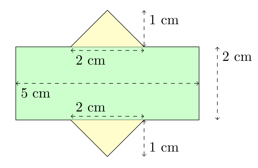
By breaking this composite shape into smaller ones, the area is at hand: $$\begin{align}A_1 &= bh = 5\cdot 2 = 10 \\ A_2 = A_3 &= \frac{bh}{2} = \frac{2\cdot 1}{2} = 1 \\ A_{total} &= A_1+A_2+A_3 = 12\end{align}$$

Unfortunately, this approach can be difficult for a person to use when they cannot physically (or mentally) see the polygon, such as when a polygon is given as a list of many vertices.

Formula

Happily, there is a formula for the area of any simple polygon that only requires knowledge of the coordinates of each vertex. It is as follows: $$A = \sum_{k=0}^{n} \frac{(x_{k+1} + x_k)(y_{k+1}-y_{k})}{2} \tag{1}$$ (Where \({n}\) is the number of vertices, \({(x_k, y_k)}\) is the \({k}\)-th point when labelled in a counter-clockwise manner, and \({(x_{n+1}, y_{n+1}) = (x_0, y_0)}\); that is, the starting vertex is found both at the start and end of the list of vertices.)

It should be noted that the formula is not “symmetric” with respect to the signs of the \({x}\) and \({y}\) coordinates. This can be explained by considering the “negative areas” incurred when adding the signed areas of the triangles with vertices \({(0,0)-(x_k, y_k)-(x_{k+1}, y_{k+1})}\).

In the next sections, I derive this formula using Green’s Theorem, show an example of its use, and provide some applications.

more »

Welcome to the Math StackExchange community blog!

Four years ago today, Dan Dumitru proposed the creation of Math.StackExchange. The site has evolved into a community with hundreds of thousands of questions and answers, and over 30 thousand questions and answers appearing each month.

Now, we have a blog.

This blog provides a way of going beyond the Q&A format to allow exposition and discussion. There might be posts about mathematics, or Math.SE, or a book review, or whatever seems appropriate. Anyone can contribute to the blog. This blog is written and edited by community members, and we are actively soliticing both one-time and regular contributors! So if you have an idea of something you’d like to hear about or read about, or if you would like to contribute, check out the blog chat room and the Blog FAQ thread on meta.

I’m looking forward to see what we make here.